econ
stor
www.econstor.eu
Der Open-Access-Publikationsserver der ZBW – Leibniz-Informationszentrum Wirtschaft
The Open Access Publication Server of the ZBW – Leibniz Information Centre for Economics
Nutzungsbedingungen:
Die ZBW räumt Ihnen als Nutzerin/Nutzer das unentgeltliche, räumlich unbeschränkte und zeitlich auf die Dauer des Schutzrechts beschränkte einfache Recht ein, das ausgewählte Werk im Rahmen der unter
→ http://www.econstor.eu/dspace/Nutzungsbedingungen nachzulesenden vollständigen Nutzungsbedingungen zu vervielfältigen, mit denen die Nutzerin/der Nutzer sich durch die erste Nutzung einverstanden erklärt.
Terms of use:
The ZBW grants you, the user, the non-exclusive right to use the selected work free of charge, territorially unrestricted and within the time limit of the term of the property rights according to the terms specified at
→ http://www.econstor.eu/dspace/Nutzungsbedingungen By the first use of the selected work the user agrees and declares to comply with these terms of use.
zbw
Leibniz-Informationszentrum WirtschaftFischer, Matthias J.; Köck, Christian; Schlüter, Stephan; Weigert, Florian
Working Paper
Multivariate Copula Models at Work:
Outperforming the desert island
copula?
Diskussionspapiere // Friedrich-Alexander-Universität Erlangen-Nürnberg, Lehrstuhl für Statistik und Ökonometrie, No. 79/2007
Provided in cooperation with:
Friedrich-Alexander-Universität Erlangen-Nürnberg (FAU)
Suggested citation: Fischer, Matthias J.; Köck, Christian; Schlüter, Stephan; Weigert, Florian (2007) : Multivariate Copula Models at Work: Outperforming the desert island copula?,
Diskussionspapiere // Friedrich-Alexander-Universität Erlangen-Nürnberg, Lehrstuhl für Statistik und Ökonometrie, No. 79/2007, http://hdl.handle.net/10419/29569
MULTIVARIATE COPULA MODELS AT WORK:
OUTPERFORMING THE ”DESERT ISLAND COPULA”?
Matthias Fischer†, Christian K¨ock\, Stephan Schl¨uter & Florian Weigert
† Department of Computational Statistics Helmut-Schmidt University of Hamburg, Germany
Email: [email protected]
\Department of Statistics and Econometrics University of Erlangen-N¨urnberg, Germany Email: [email protected]
This research was kindly supported by the Hans Frisch-Stiftung.
summary
Since the pioneering work of Embrechts and co-authors in 1999, copula models enjoy steadily increasing popularity in finance. Whereas copulas are well-studied in the bivariate case, the higher-dimensional case still offers several open issues and it is by far not clear how to construct copulas which sufficiently capture the characteristics of financial returns. For this reason, elliptical copulas (i.e. Gaussian and Student-t copula) still dominate both empirical and practical ap-plications. On the other hand, several attractive construction schemes appeared in the recent literature promising flexible but still manageable dependence mod-els. The aim of this work is to empirically investigate whether these models are really capable to outperform its benchmark, i.e. the Student-tcopula (which is termed by Paul Embrechts as ”desert island copula” on account of its excellent fit to financial returns) and, in addition, to compare the fit of these different copula classes among themselves.
Keywords and phrases: KS-copula; Hierarchical Archimedian; Product copulas; Pair-copula decomposition
1
Introduction
The increasing linkages between countries, markets and companies require an accurate and realistic modelling of the underlying dependence structure. This applies to financial markets and, in particular, to the financial assets traded there-on. For a long time both practitioners and theorists rely on the multivariate normal (Gaussian) distribution as statistical funda-ment, seemingly ignoring that this model assigns too less probability mass to extremal events. In order to remove this drawback but still maintain many of the attractive proper-ties, elliptical distributions (e.g. multivariate Student-t or multivariate generalized hyper-bolic distribution) occasionally found its way into financial literature. Though being able to model heavy tails, elliptical distributions fail to capture asymmetric dependence struc-tures. The copula concept, in contrast, which originally dates back to Sklar (1959) but was made popular to finance through the pioneering work of Embrechts and co-authors (1999)
provides a flexible tool to capture different patterns of dependence. Within this work we assume that the reader is already familiar with the notion of copulas. Otherwise, we refer to Nelsen (2006) or Joe (1997). Whereas copulas are well-studied in the bivariate case, con-struction schemes for higher dimensional copulas are not. Recently, several publications on high-dimensional copulas appeared (e.g. Morillas, 2005, Palmitesta & Provasi, 2005, Savu & Trede, 2006, Liebscher, 2006, Aas et al., 2006). Each of them claims to provide a flexible dependence model, but there is no comprehensive comparison among these approaches, as far as we know. In particular, no references are found to the Student-t copula (i.e. the copula associated to the multivariate Student-t distribution) which is sometimes termed as ”desert island copula” by Paul Embrechts on account of its excellent fit to multivariate financial return data.
The outline of this work is as follows: Section 2 overviews and connects several recent construction schemes of multivariate copulas. A short digression on goodness-of-fit measures can be found in section 3. Section 4 is dedicated to the description of the underling data sets, whereas the empirical results are summarized and discussed in section 5.
2
Constructing multivariate non-elliptical copulas
Among the classes of non-elliptical copulas, Archimedean copulas and its generalizations (section 2.1) enjoy great popularity. Above that, so-called pair-copula constructions are re-viewed in section 2.2, where the joint distribution is decomposed into simple building blocks, so-called pair-copulas. Thirdly, we pick up the copulas associated to K¨ohler-Symanowski distributions in section 2.3 which have been successfully applied by Palmistesta & Provasi (2005) as models for financial returns. Finally, Liebscher’s (2006) recent proposal to gener-alize givend-copulas is reviewed in section 2.4.
2.1
Multivariate Archimedean copulas
2.1.1 Classical multivariate Archimedean copulasLetϕ: [0,1]→[0,∞] be a continuous, strictly decreasing and convex function withϕ(1) = 0,
ϕ(0)≤ ∞and letϕ[−1] be the so called pseudo-inverse ofϕdefined by
ϕ[−1](t)≡ ϕ−1(t) 0≤t≤ϕ(0), 0 ϕ(0)≤t≤ ∞.
It can be shown (see, e.g. Nelsen, 2006) that
C(u1, u2) =ϕ[−1]
ϕ(u1) +ϕ(u2)
defines a class of bivariate copulas, the so-called Archimedean copulas. The functionϕ is called the (additive) generator of the copula. Furthermore, ifϕ(0) =∞the pseudo-inverse
describes an ordinary inverse function (i.e. ϕ[−1] =ϕ−1) and in this case ϕis known as a strict generator.
Given a strict generatorϕ: [0,1]→[0,∞], bivariate Archimedean copulas can be extended to thed-dimensional case. For everyd≥2 the functionC: [0,1]d→[0,1] defined as
C(u) =ϕ−1ϕ(u1) +ϕ(u2) +· · ·+ϕ(ud)
(2.1) is ad-dimensional Archimedean copula if and only if ϕ−1 is completely monotonic on
R+, i.e. ifϕ−1∈ L∞with Lm≡ n φ:R+→[0,1] φ(0) = 1, φ(∞) = 0,(−1) kφ(k)(t)≥0, k= 1, . . . , m,o. The Gumbel copula derives from the generator ϕ(t) = (−lnt)θ, θ ≥ 1 and the Clayton
copula is generated by ϕ(t) = 1θ(t−θ−1), θ >0. For an overview of further Archimedean copulas and the properties of the aforementioned ones, we refer the reader to the monographs by Nelson (2006) and Joe (1997).
2.1.2 Non-exchangeable Archimedean copulas
In order to increase flexibility and to allow for non-exchangeable dependence structures, sev-eral gensev-eralizations emerged in the recent literature: A simple one – the so-called fully nested Archimedean (FNA) copulas – can be found in Joe (1997, p. 89), Whelan (2004) and Savu & Trede (2006), and requiresd−1 generator functionsϕ1, . . . , ϕd−1withϕ−11, . . . , ϕ
−1 d−1∈ L∞ andϕi+1◦ϕ−i1(t) =ϕi+1(ϕ−i 1(t))∈ L∗∞for L∗ d= n φ:R+→R+ φ(0) = 0, φ(∞) =∞,(−1) k−1φ(k)(t)≥0, k= 1, . . . , d,o. The structure of FNA d-copulas is rather simple: One first couples u1 and u2. One then couples the copula ofu1 andu2 withu3to a new copula which is coupled afterwards with
u4and so on. Hence the FNA 4-copula is of the form
C(u) =ϕ−31
ϕ3 ϕ−21
ϕ2 ϕ−11[ϕ1(u1) +ϕ1(u2)]+ϕ2(u3)+ϕ3(u4). (2.2)
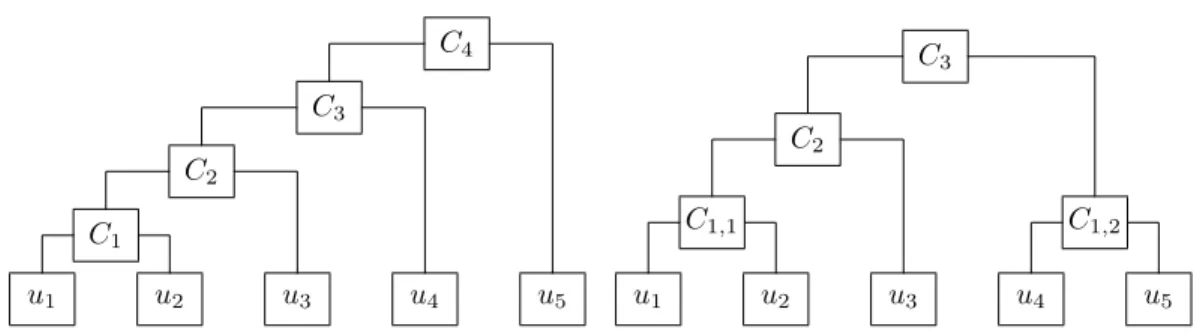
Figure 1 illustrates one possible FNA copula for dimensiond= 5.
Secondly, mixing ordinary Archimedean and FNA copulas, partially nested Archimedean (PNA) copulas may be used. Again, for ease of notation, we focus on the 4-variate case
C(u) =ϕ−1 ϕ ϕ−121[ϕ12(u1) +ϕ12(u2)] +ϕ ϕ−341[ϕ34(u3) +ϕ34(u4)] . (2.3)
Note thatϕ, ϕ12, ϕ34 are generators withϕ−1, ϕ−121, ϕ
−1
34 ∈ L∞ andϕ◦ϕ−121, ϕ◦ϕ
−1 34 ∈ L∗∞. Obviously, one first couples the pairsu1, u2andu3, u4with distinct generators. The resulting copula pair is then coupled using a third generatorϕ(which in turn might be coupled with
u1 u2 u3 u4 u5 C1 C2 C3 C4 u1 u2 u3 u4 u5 C1,1 C1,2 C2 C3
Figure 1: FNA copula (left) and PNA copula (right) ford= 5.
an additional variableu5 using a fourth generatorψ for an extension to the 5-dimensional case). Another possible structure of a PND copula is illustrated in figure 1.
Thirdly, copula C from (2.3) is also an example of a so-called hierarchical Archimedean (HA) copulas. The basic idea of this approach (see, e.g. Savu & Trede, 2006) is to build a hierarchy of Archimedean copulas. Let there be L hierarchy levels indexed byl. At each level l= 1, . . . , L one has nl distinct objects with index j= 1, . . . , nl. The u1, . . . , ud are
located at the lowest level,l= 0. At levell= 1 theu1, . . . , udare grouped inton1 ordinary multivariate Archimedean copulasC1,j,j= 1, . . . , n1, of the form
C1,j(u1,j) =ϕ−1,j1
X
ϕ1,j(u1,j)
where ϕ1,j denotes the generator of copula C1,j. Let u1,j denote the set of elements of
u1, . . . , ud belonging to copula C1,j for j= 1, . . . , n1. The copulas C1,1, . . . , C1,n1 might belong to different Archimedean families. All copulas of levell = 1 are in turn aggregated into copulas at levell= 2. Then2 copulasC2,j,j= 1, . . . , n2are generalized Archimedean copulas, whose dependence structure is only of partial exchangeability. They consist of copulas from the previous level (as elements) and can be represented as
C2,j(C2,j) =ϕ−2,j1 X C2,j ϕ2,j(C2,j) ,
where ϕ2,j denotes the generator of copulaC2,j, andC2,j represents the set of all copulas
from levell= 1 entering copulaC2,j forj= 1, . . . , n2. We can proceed in this manner until attaining levelLwith the hierarchical Archimedean copulaCL,1 as single object.
In order to ensure that CL,1 is a proper copula, we have to proclaim that ϕ−l,j1 ∈ L∞ for l= 1, . . . , L and j= 1, . . . , nl, and that ϕl+1,i◦ ϕ−l,j1 ∈ L
∗
∞ for all l= 1, . . . , L and
j= 1, . . . , nl,i= 1, . . . , nl+1such thatCl,j ∈Cl+1,i. Moreover, a hierarchy is established if
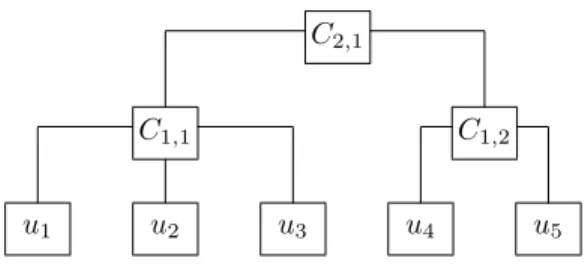
the number of copulas decreases at each level, if the top level contains only a single object and if at each level the dimensions of the copulas add up tod. Figure 2 displays the possible construction of a 5-dimensional HA-copula.
u1 u2 u3 u4 u5
C1,1 C1,2
C2,1
Figure 2: HA copula ford= 5.
Savu & Trede (2006) also derive the HA-copula density
∂dCL,1 ∂u1. . . ∂ud =X ∂ d−iC L,1 ∂Ck1 L−1,1. . . ∂C kn,L−1 L−1,nL−1 nL−1 Y r=1 X u=υ1,...,υr ∂|υ1|C L−1,r ∂υ1 , . . . ,∂ |υr|C L−1,r ∂υr ,
where the outer sum extends over all sets of integers k1, . . . , kn,L−1 ∈ N0 such that maxj
kj ≤dL−1,j and P nL−1
j=1 kj =d−i for all i= 0, . . . , d−nL−1. These terms are the outer derivatives of the copula with respect to the elements ofCL,1, i.e., thenL−1 copulas from levelL−1. The second part of the formula are the inner derivatives, corresponding to the derivatives of the copulas at levelL−1 with respect to their arguments uL−1,j.
2.1.3 Generalized multiplicative Archimedean copulas
In this section we focus on methods recently proposed by Morillas (2005) and Liebscher (2006). Both approaches are based on a second functional representation of Archimedean copulas via so called multiplicative generators (see Nelsen, 2006). Settingϑ(t)≡exp(−ϕ(t)) andϑ[−1](t)≡ϕ[−1](−lnt), equation (2.1) can be rewritten as
C(u1, . . . , ud) =ϑ[−1]
ϑ(u1)·ϑ(u2)·. . .·ϑ(ud)
. (2.4)
The functionϑ is called multiplicative generator of C. Due to the relationship between ϕ
and ϑ, the function ϑ : [0,1] → [0,1] is continuous, strictly increasing and concave with
ϑ(1) = 1 andϑ[−1](t) = 0 if 0≤t≤ϑ(0) andϑ[−1](t) =ϑ−1(t) ifϑ(0)≤t≤1. Equation (2.4) can also be expressed using the independence copulaC⊥(u) =Qd
i=1ui: C(u1, . . . , ud) =ϑ[−1] C⊥(ϑ(u1), . . . , ϑ(ud)) .
Morillas (2005) substitutesC⊥ by an arbitraryd-copulaC in order to obtain
Cϑ(u1, . . . , ud) =ϑ[−1]
C(ϑ(u1), ϑ(u2), . . . , ϑ(ud))
(2.5) and proves thatCϑ is ad-copula ifϑ[−1] isabsolutely monotonic of order don [0,1], i.e. if
ϑ[−1](t) satisfies (ϑ[−1])(k)(t) =dkϑ[−1](t)
Examples of generator functions are stated in Morillas (2005). Notice that not every gen-erator given there is absolutely monotonic for arbitrary d > 1: As one can easily verify, the generator ϑ(t) =tr/(2−tr), r ∈(0,1/3] (see table 1, no. 9 in Morillas, 2005) has no absolutely monotonic pseudo-inverse of order d≥ 3, because the third derivative ofϑ[−1] becomes negative. Hence this generator is suitable only for a construction of generalized bivariate copulas. Concerning the basic properties of such Morillas copulas we refer to Mo-rillas (2005).
Another way of generalizing Archimedean copulas is the method proposed by Liebscher (2006) who introduces the following copula representation
C(u1, . . . , ud) = Ψ 1 m m X j=1 ψj1(u1)·ψj2(u2)·. . .·ψjd(ud) , (2.6)
where Ψ and ψjk : [0,1]→ [0,1] are functions satisfying the following conditions: Firstly,
it is assumed that Ψ(d) exist with Ψ(k)(u)≥0 for k = 1,2, . . . , dand u∈ [0,1], and that Ψ(0) = 0. Secondly, ψjk is assumed to be differentiable and monotone increasing with
ψjk(0) = 0 andψjk(1) = 1 for allk, j. Thirdly, Liebscher’s construction requires that
Ψ 1 m m X j=1 ψjk(v) =v for k= 1,2, . . . , dandv∈[0,1].
The three conditions guarantee thatC defined in (2.6) is actual a copula.
It is easily seen that the approaches of Morillas (2005) and Liebscher (2006) coincide for
m= 1, ϑ[−1]= Ψ in (2.6) andCϑ=C⊥ in (2.5).
Liebscher (2006) also states a general method for deriving appropriate functions ψjk. Let
hjk: [0,1]→[0,1], j= 1, . . . , m, k= 1, . . . , dbe a differentiable and bijective function such
that h0jk(u) > 0 for u ∈ (0,1), hjk(0) = 0, hjk(1) = 1 and mu = P m
j=1hjk(u), u ∈
[0,1], k= 1, . . . , d. Letψ= Ψ−1be the differentiable inverse function of Ψ. An appropriate choice is settingψjk(u) =hjk(ψ(u)), sinceψ0jk(u) =h
0 jk(ψ(u))·ψ 0(u)>0 forj = 1, . . . , m andu∈[0,1]. Consideringm= 2, define h1k(u)≡uδk, h2k(u)≡2u−uδk with δk ∈[1,2]. (2.7) Choosing further Ψ(t) =−1 θln(1−(1−e −θ )t), and ψ(u) =1−e −θu 1−e−θ , θ >0
and definingψjk(u)≡hjk(ψ(u)) a generalized Frank copula (GMLF) is obtained. Setting
the common Frank copula. Settingm= 2 and hjk as in (2.7) but now choosing (see table 2, no. 2, p. 8 in Liebscher (2006)) Ψ(t) = (δ−t) −θ−δ−θ (δ−1)−θ−δ−θ, and ψ(u) =δ− δ −θ(1−u) +u(δ−1)−θ−1θ, θ >0, δ >1 a copula is obtained, which will be termed as GML2 copula henceforth.
In the field of insurance pricing the function ψjk is known as a distortion function (for a
definition see Freez & Valdez, 1998) and the methods proposed by e.g. Freez & Valdez (1998) or Wang (1998) appear as special cases in (2.6). The same holds for the approach given by Morillas (2005) where the functionϑalso satisfies the requirements of a distortion function.
2.2
Pair-copula decompositions
2.2.1 Pair-copula decomposition: The general case
One way of calculating a multivariate density is by decomposing it into a product of marginal densities and conditional densities. The latter can be stepwise replaced by so-called pair-copulas. Again, letX= (X1, . . . , Xd)0 have the joint density function
f(x1, . . . , xd) =f(xd)·f(xd−1|xd)·f(xd−2|xd−1, xd)·. . .·f(x1|x2, . . . , xd) (2.8)
which is unique up to a relabelling of the variables. Because of
f(x1, . . . , xd) =c12···d(F1(x1), . . . , Fd(xd))·f1(x1)· · ·fd(xd),
withc12···d(·) being thed-variate copula density,f(xd|xd−1), e.g., may also be expressed by
c12(F1(x1), F2(x2))·f1(x1). c12(·,·) is called pair-copula density for the respecting trans-formed variables. f(xd−2|xd−1, xd), again, can be decomposed into
c(d−2)d|d−1 Fd−2|d−1(xd−2|xd−1), Fd|d−1(xd, xd−1) ·f(xd−2|xd−1). Usingf(xd−2|xd−1) =c(d−2)(d−1)(Fd−2(xd−2), Fd−1(xd−1))·fd−2(xd−2) results in f(xd−2|xd−1, xd) = c(d−2)d|d−1(Fd−2|d−1(xd−2|xd−1), Fd|d−1(xd, xd−1)) · c(d−2)(d−1)(Fd−2(xd−2), Fd−1(xd−1))·fd−2(xd−2).
But this is not unique anymore, because, while splitting up, conditioning onxd instead of
xd−1 is also possible. This leads to a different decomposition. Thegeneral formula reads
f(x|v) =cxvj|v−j(F(x|v−j, F(vj|v−j))·f(x|v−j) (2.9) for ad-dimensional vector v with componentsvj. v−j denotesv excluding the component
As seen above, every (conditional)d-dimensional density can be split up into a pair-copula and a (d−1)-dimensional (conditional) density. For d >2 you can iteratively repeat this splitting for the (d−1)-dimensional conditional density. Eventually, you will get a product of univariate densities and pair-copulas. Like shown in the trivariate case, this decomposi-tion is not unique but there are various ways to do so.
In order to sort the different decomposition constructs, so-calledregular vines (see Bedford and Cooke, 2001 and 2002) are defined. Vines are graphical models that present complete decomposition schemes. Following Aas et al. (2006) we choose the structure of the D-vine, since there is no dominating variable. The joint densityf(x1, . . . , xd) can be expressed as
d Y k=1 f(xk) d−1 Y j=1 d−j Y i=1 ci,i+j|i+1,...,i+j−1(F(xi|xi+1, . . . , xi+j−1), F(xi+j|xi+1, . . . , xi+j−1)). The decomposition of a four-dimensional density according to the D-vine scheme is
f(x1, x2, x3, x4) = f(x1)·f(x2)·f(x3)·f(x4)
·c12(F(x1), F(x2))·c23(F(x2), F(x3))·c34(F(x3), F(x4))
·c13|2(F(x1|x2), F(x3|x2))·c24|3(F(x2|x3), F(x4|x3))
·c14|23(F(x1|x2, x3), F(x4|x2, x3)). (2.10) 2.2.2 Pair-copula decomposition of a copula
Originally, the pair-copula decomposition (PCD) decomposes the common density f of d
random variables. Of course, one may also apply the pair-copula decomposition to the underlying copula density c, as we will show in this subsection. To simplify notation, we restrict ourselves tod= 4 and the D-vine decomposition. As an immediate consequence of Sklar’s (1959) theorem,
c(F(x1), F(x2), F(x3), F(x4)) =
f(x1, x2, x3, x4)
f(x1)·f(x2)·f(x3)·f(x4)
.
Substituting the common density by its PCD given in (2.10),
c(F(x1), F(x2), F(x3), F(x4)) = c12(F(x1), F(x2))·c23(F(x2), F(x3))·c34(F(x3), F(x4))
·c13|2(F(x1|x2), F(x3|x2))·c24|3(F(x2|x3), F(x4|x3))
·c14|23(F(x1|x2, x3), F(x4|x2, x3))
with ci|j(·,·) being a pair-copula density and its indicesi, j refer to xi andxj. According
to Joe (1996),
F(x|v) = ∂ Cx,vj|v−j(F(x|v−j), F(vj|v−j))
withv−j being the vectorvexcept the elementvj. In the univariate case (i.e. v=v),
F(x|v) =∂ Cx|v(FX(x), FV(v))
∂ FV(v)
≡h(x, v, θ),
whereθ being the parameter vector of the copulaCx,v. The copula density decomposition
can be written as follows: It is obvious that F(x1|x2) = h(x1, x2, θ12) with θ12 is the parameter (vector) of the of copulaC12. Analogously,F(x3|x2) =h(x3, x2, θ23),F(x2|x3) =
h(x2, x3, θ23) andF(x4|x3) =h(x4, x3, θ34). F(x1|x2, x3), again, can be iteratively simplified to
∂ C13|2(F(x1|x2), F(x3|x2))
∂ F(x3|x2)
=h(h(x1, x2, θ12), h(x3, x2, θ32), θ13|2).
Analogously,F(x4|x2, x3) can be written as
∂ C24|3(F(x4|x3), F(x2|x3))
∂ F(x2|x3)
=h(h(x4, x3, θ43), h(x2, x3, θ23), θ24|3).
Finally, define u1 = F(x1), u2 = F(x2), u3 = F(x3), u4 = F(x4). The formula for the 4-dimensional PCD copula density now reads as
c(u) = c12(u1, u2)·c23(u2, u3)·c34(u3, u4)
·c13|2(h(u1, u2, θ12), h(u3, u2, θ23))· c24|3(h(u2, u3, θ23), h(u4, u3, θ34))
·c14|23(h(h(u1, u3, θ13), h(u2, u3, θ23), θ13|2), h(h(u4, u3, θ43), h(u2, u3, θ23), θ24|3)) To summarize, in order to specify a d-dimensional (copula) density, two main steps have to be taken (see Aas et al., 2006): Firstly, an appropriate decomposition scheme has to be selected as follows: use the canonical vine scheme, if there is a key-variable. If not, use the D-vine scheme. Secondly, the pair-copulas have to be specified: e.g. Gaussian, Student’st, Archimedean or Gumbel copula. It is possible, to use one copula model for all pair-copulas or decide individually.
2.3
Koehler-Symanowski (KS) copulas
Koehler & Symanowski (1995) introduce a multivariate distribution as follows: With the index setV ={1,2, . . . , d},V being the power set ofV andI ≡ {I∈ Vwith|I| ≥2}letX denote ad-dimensional random vector with univariate marginal distributionsFi(xi), i∈V.
For all subsetsI∈ IletαI ∈R0+andαi ∈R+0 for alli∈V such thatαi+=αi+PI∈IαI >0
fori∈I. Then the common cdfF is defined by
F(x1, . . . , xd) = Q i∈V Fi(xi) Q I∈I h P i∈I Q j∈I,j6=iFj(xj)αj+−(|I| −1)Qi∈IFi(xi)αi+ iαI . (2.11) The terms KI =Pi∈I Q
j∈I,j6=iFj(xj)αj+−(|I| −1)Qi∈IFi(xi)αi+ are called association
exists if the marginal density functions fi exist for all i ∈ V. Due to the design of the
Koehler-Symanowski distribution the corresponding copula has a similar functional form: Settingui=Fi(xi) for alli∈V, the KS copula is
C(u1, . . . , ud) = Q i∈V ui Q I∈I h P i∈I Q j∈I,j6=iu αj+ j −(|I| −1) Q i∈Iu αi+ i iαI . (2.12)
In contrast to the cumulative distribution function the functional representation of the density is quite complicated due to complex factors with additive components. Koehler & Symanowski (1995) gave an explicit formula for the special case of a so called KS(2)-distribution (Caputo, 1998), where all parameters αI are set equal zero for |I| > 2. The
corresponding copula will be termed as KS(2) copula henceforth. Assuming that αij ≡
αji ≥ 0 for all (i, j) ∈ V ×V and αi+ = αi1+αi2+· · ·+αid > 0 for all i ∈ V, the
KS(2)-copula simplifies to C(u1, u2, . . . , ud) = d Y i=1 ui Y i<j Y K−αij ij (2.13) withKij≡u 1/αi+ i +u 1/αj+ j −u 1/αi+ i u 1/αj+ j =Kji.
Palmitesta & Provasi (2005) apply this particular KS copula to weekly log-returns. They also argue that this copula has the ability to model complex dependence structures among subsets of marginal distribution but they do not present any goodness-of-fit measure or any comparison with other copulas. We seize the proposal by Palmitesta & Provasi but set the association parameterαI ≥0 for|I|= 2 and|I|= 4 in (2.12), while all parametersαI are
set equal to zero for|I|= 3, i.e. we include a global dependence parameter and refer to this copula as augmented KS(2) copula (aKS(2)). Additionally, we use the KS-Copula (KSC) as defined in (2.12).
2.4
Multiplicative Liebscher copulas
By now, different methods have been reviewed how to constructd-variate copulas. Liebscher (2006), in contrast, discusses how to combine or connect a given set ofkpossibly different
d-copulas C1, . . . , Ck to a newd-copula C in order to increase flexibility and/or introduce
asymmetry. His proposal focusses on multiplicative connections ofd-copulas of the form
C(u1, . . . , ud) = k
Y
j=1
Cj(gj1(u1), . . . , gjd(ud)) (2.14)
with a set of k·d admissible functions g11, . . . , g1d, . . . , gk1, . . . , gkd, each of which being
bijective, monotonously increasing or identically equal 1 satisfying
k
Y
j=1
Note that (2.15) reduces to g1i(v) = v for k= 1 and i = 1, . . . , d, and C is recovered. In
accordance to Liebscher (2006), possible choices are
gji(v)≡vθji withθji>0 and k X j=1 θji= 1 fori= 1, . . . , d (2.16) g1i(v) =f(v), g2i(v)≡v· 1 f(v), f(v) = 1 −e−θiv 1−e−θi α , θ >0, α∈(0,1) (2.17) We consider four different generalized Clayton copulas based on (2.14). The ”Generalized Clayton of Liebscher type I” (L1) is obtained by setting k= 2, choosing the clayton copula forC1, the independence copula forC2andgji(v) as in (2.16). Applying (2.17) rather than
(2.16), the ”Generalized Clayton of Liebscher type II” (L2) copula with d+ 2 dependence parameters is constructed. Similarly, combining twod-variate Clayton copulas and usingg
from (2.16) we obtain the d-dimensional copula family with d+ 2 parameters, termed as the ”Generalized Clayton of Liebscher type III” (L3) in the sequel. Finally, applying again (2.17) rather than (2.16), the ”Generalized Clayton of Liebscher type IV” (L4) is obtained.
3
Goodness-of-fit measures
We now tackle the problem to compare the goodness-of-fit (GOF) of the different copula models from section 2, noting that most of them are not nested. As we apply maximum likelihood (ML) methods to obtain estimators for the unknown parameter vector, the first choice is the log-likelihood value`or – in order to take the different numbers of parameters in account – the information criterion of AkaikeAIC =−2`+ (2N(K+ 1))/(N−K−2), where K and N denote the number of parameters to be fitted and the number of obser-vations, respectively. However, comparing log-likelihood values for non-nested models may produce misleading conclusions. Therefore, certain GOF tests may come to application. Following Breymann, Dias & Embrechts (2003), Chen, Fan & Patton (2004) or recently Berg & Bakken (2006), the main idea is to project the multivariate problem into a set of independent and uniformU(0,1) variables, given the multivariate distribution and to calcu-late the distance (e.g. Anderson-Darling, Kolmogorov-Smirnov, Cram´er-von Mises, Kernel smoothing) between the transformed variables and the uniform distribution. In contrast to the authors above, we are not primarily interested whether the data stem from the specified copula model but we use these distances as citerion itself. The proceeding is roughly as follows:
By means of the Rosenblatt (1952) transformation the random vectorX= (X1, . . . , Xd)0 is
mapped onto a random vectorZ∗= (Z1∗, . . . , Zd∗)0 via
It can be shown thatZ∗ is uniformly distributed on [0,1]d with independent components
Z1∗, . . . , Zd∗. Assume that the cumulative distribution function ofX admits the decomposi-tion
FX(x1, . . . , xd) =C(FX1(x1), . . . , FXd(xd)),
whereC(·) denotes a parametric copula which is the common distribution function ofU= (U1, . . . , Ud)0 withUi ≡FXi(Xi). DefineC(u1, . . . , uj)≡C(u1, . . . , uj,1, . . . ,1) forj ≤d. Furthermore, the conditional distribution ofUi|U1, . . . , Ui−1 is given by
Ci(ui)≡ ∂i−1C(u1, . . . , ui) ∂u1. . . ∂ui−1 .∂i−1C(u1, . . . , ui−1) ∂u1. . . ∂ui−1 .
According to (3.1), the variables
Z1≡C(U1) =U1 and Zi≡Ci(Ui), i= 2, . . . , d (3.2)
are independent and uniform on [0,1]. Consequently, the sampleX1, . . . ,XN from a
para-metric copula and with marginals given byF1, . . . , Fd can be mapped onto an iid sample
Z1, . . . ,ZN from a uniform distribution on [0,1]d.
Breymann et al. (2003) suggest to transform each random vectorZi= (Zi1, . . . , Zid)0 in a
(univariate) chi-square variableχj withddegrees of freedom throughχj =P d i=1Φ−
1(Z
ji)2,
j= 1, . . . , N,where Φ−1(u) denotes the standard normal quantile function. If the margins are unknown, they may be replaced by the corresponding empirical counterparts. Breymann et al. state that ”we do assume that theχ2-distribution will not be significantly affected by the use of the empirical distribution functions used to transform the marginal data”.
4
The data set
The data sets we used used to compare the different copula models come from three dif-ferent markets (German stock market, foreign exchange (FX) market and commodity mar-kets). From each market, four typical representatives were selected, provided that the corresponding sample period is sufficiently large. Instead of analyzing the prices them-selves, we calculated and considered (percentual) continuously compounded returns (”log-returns”) Rt = 100(logPt−logPt−1), t = 2, . . . , N. In order to account for possible time-dependencies (which are common to most financial return series), we also fitted uni-variate GARCH models of the formRt=µ+γ1Rt−1+. . .+γkRt−k+htt with variance
equations h2t =α0+α1R2t−1+. . .+α1Rt2−p+β1h2t−1+. . .+βqh2t−q to each of the series
and considered standardized residualstrather the original returnsRt. Secondly, as we are
primarily not interested in parametric models for the marginal distributions, all observations (i.e. returns or standardized residuals) were transformed into uniform ones by means of the (empirical) probability integral transform, i.e.
Ut=FN(Rt) withFN(x) =
{#Rt|Rt≤x}
#Rt
4.1
German stock returns
From the German stock market, we selected prices of HVB AG, BMW AG, Allianz AG and Munich Re AG, all of them being part of the German stock market index DAX which measures the performance of the Prime Standard’s 30 largest German companies in terms of order book volume and market capitalization. Figure 3 contains the series of prices and returns. Table 1 summarizes descriptive and inductive statistics. All series feature negative
Figure 3: German stock prices and stock returns.
skewness and high kurtosis (measured by the third and fourth standardized momentSand K). Morerover, there is empirical evidence for (slight) serial correlation and GARCH effects as the Ljung-Box statisticLB and Engle’s Lagrange multiplier statisticLMindicate.
Start End N Stocks µ s2
S K LB(10) LM(10) 02-01-90 12-11-03 3486 HVB 0.004 5.61 -0.033 8.16 24.45 621.08 02-01-90 12-11-03 3486 BMW 0.046 4.33 -0.132 7.19 28.96 366.49 02-01-90 12-11-03 3486 Allianz -0.002 4.87 -0.07 8.37 29.74 517.14 02-01-90 12-11-03 3486 MunichRe 0.02 5.06 -0.027 8.75 50.53 508.59
Table 1: German stock returns.
4.2
Exchange rate returns
Data from foreign exchange markets (FX-markets) are available from the PACIFIC Ex-change Rate Service1. This service offered by Prof. Werner Antweiler at UBC’s Sauder School of Business provides access to current and historic daily exchange rates through an on-line database retrieval and plotting system. In contrast to the volume notation, where values are expressed in units of the target currency per unit of the base currency, the price
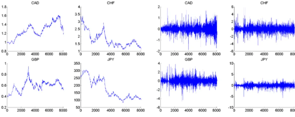
notation is used within this work which corresponds to the numerical inverse of the volume notation. All values are expressed in units of the base currency (here US-Dollar) per unit of the target currency. Table 2 summarizes the statistics of the four exchanges rates (Canadian Dollar, Japanese Yen, Swiss Franc, British Pound) which are used later on. Again, prices and log-returns in figure 4, below.
Figure 4: Exchange rates: Prices versus Returns.
Start End N FX Rate µ s2
S K LB(10) LM(10) 02-01-90 31-12-04 3794 CAD 0.002 0.09 -0.004 6.75 12.65 912.18 02-01-90 31-12-04 3794 YEN -0.015 0.56 -0.002 6.11 12.5 429.24 02-01-90 31-12-04 3794 SFR 0.003 0.36 0.132 6.84 55.79 485.26 02-01-90 31-12-04 3794 BRP -0.013 0.44 -0.723 13.33 34.48 176.20
Table 2: Exchange rates
4.3
Metal returns
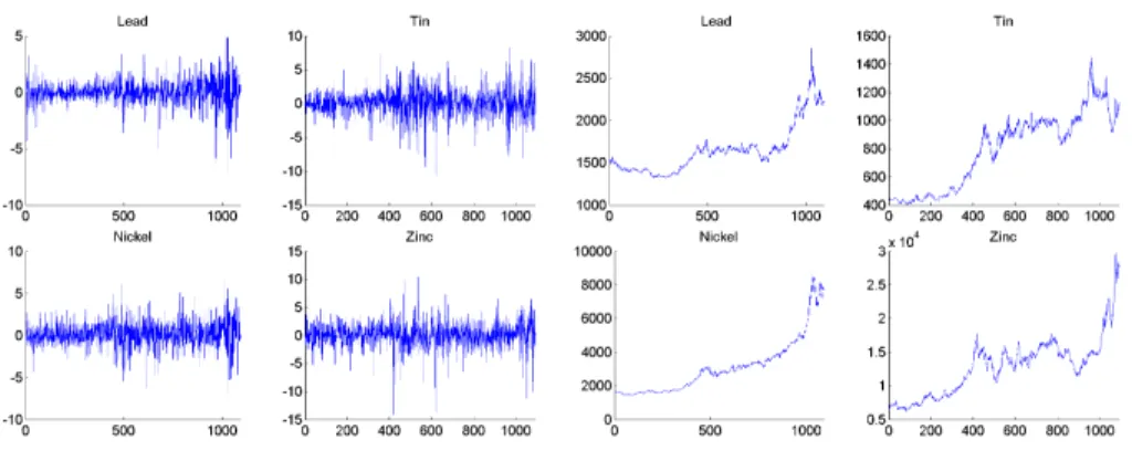
The London Metal Exchange2(LME) is the world’s premier non-ferrous metals market with a turnover value of some US$2000 billion per annum. For a detailed introduction on metal markets with emphasis on the London metal exchange see Crowson & Sampson (2001). Among the different metals, emphasis is placed on aluminium, copper, lead and nickel. All prices are quoted in US-Dollar per tonne. Table 3 contains again the basic summary statistics. Prices and log-returns are displayed in figure 5.
Figure 5: Metals: Prices versus Returns.
Start End N Metal µ s2
S K LB(10) LM(10)
26-03-99 07-08-06 1093 Lead 0.034 1.22 -0.555 8.72 29.74 161.56 26-03-99 07-08-06 1093 Tin 0.084 4.21 -0.368 5.59 30.11 100.37 26-03-99 07-08-06 1093 Nickel 0.142 2.38 -0.139 5.13 12.95 127.66 26-03-99 07-08-06 1093 Zinc 0.13 4.97 -0.618 7.9 10.72 21.45
Table 3: Metals: Prices versus Returns.
5
Empirical results
The 4-copulas under consideration are the following: Firstly, we selected the Clayton copula (CLA), the Gumbel copula (GUM) and its rotated version (roGUM) from the Archimedean class. From the generalized Archimedean copula family, two hierarchical copula models (i.e. HA-CLA and HA-GUM) are included, based on the Clayton and the Gumbel copula, re-spectively. Moreover, six representatives of Morrillas’ construction scheme (i.e. MO-CLA1, MO-CLA2, MO-CLA3, MO-GUM1, MO-GUM2, MO-GUM3) involving the Clayton, the Gumbel and different generator functions (no. 3, 2, 4 in Morillas, 2005) are included as well. In addition, two version of Liebscher’s proposal (GMLF, GML2) are used. Above that, representing the ”elliptical copula world”, the Gaussian copula (NORM) and – as ultimate benchmark – the Student-t (T) copula are also included. From the pair-copula decomposition we chose five representatives (i.e. PC-NORM, PC-T, PC-CLA, PC-GUM, PC-roGUM) each of them derived from one single copula model (i.e. we used no decom-positions based on different copulas). Finally, the KS(2)-copula and its augmented version (which is a generalized version of Palmitesta & Provasi, 2005 because we included a general dependence parameter) and four different types of multiplicative Liebscher copulas from example 2.8 (L1,L2,L3,L4) are considered.
The computer code for the ML-estimation was implemented in Matlab 7.1. For maximiza-tion purposes we used the line-search algorithm of Matlab. The following tables include the comprehensive results for the parameter estimates as well as the different goodness-of-fit measures for all data sets (returns and GARCH-residuals) and all copulas models men-tioned above. As stated above, goodness-of-fit is measured by the Log-likelihood value and Akaike’s AIC criterion. Above that, two distance measures,
KS =√N max j=1,...,N Fχ2(d)(χj)−FN,χ(χj) and AKS = √1 N X j=1,...,N Fχ2(d)(χj)−FN,χ(χj)
are calculated to quantify the distance after application of the Rosenblatt transformation (based on the different parametric copula models).
The estimation results are unique across the different data set. As known from several em-pirical studies, the fit of the 4-variate Gaussian distributions may be considerably improved if the 4-variate Student-t distribution is considered, instead. However, pair-copula decom-positions based on bivariate Student-tcopulas produce a similar goodness-of-fit, sometimes even outperform the 4-variate Student-t distribution. Whereast-PCD dominate the likeli-hood criteria, 4-variate Student-t distribution provide minimal distance measure in many cases. Similar, PCD-decompositions based on Archimedean copulas may also be considered as possible alternatives. This also applies to the three copulasL1,L3 andL4, in particular for the exchange rate data, whereas all copulas based on Morillas’ approach and, of course, the plain Archimedean copulas feature low goodness-of-fit measures. Considering hierarchi-cal Archimedean copulas, instead, we found only slight improvement, at least for our data sets. However, we have to confess that one might improve the results with another hierarchy which might be found on the basis of cluster algorithms.
The KS(2)-copula (recommended by Palmitesta and Provasi, 2005) provides only a poor fit to the return series. However, introducing an additional dependence parameter – which quantifies the overall dependence in the data set – clearly improves all goodness-fit measures. Above that, removing the GARCH effects found in the margins doesn’t change the esti-mation results substantially. In particular, the ordering of the goodness-of-fit measures is essentially preserved. Above that, parameter estimates of the dependence parameters are roughly stable for most of the copulas under consideration.
To sum up, the 4-variate Student-t distribution still plays a predominant role. Some of the recently proposed construction schemes are partially competitive while others are more likely to be overestimated in the literature.
Germa n sto c ks (G AR CH-Res idual s) Ex c h ange r ates (G AR CH-Res iduals) Metal (G AR CH-Res iduals) Copula l AI C K S AK S l AI C K S AK S l AI C K S AK S CL A 1847. 1 -3 690.2 5. 90 0. 89 1780. 5 -35 56.9 5. 53 0. 89 425. 9 -84 7.8 1. 64 0. 26 GU M 1835. 0 -3 666.0 4. 87 0. 85 1787. 1 -35 70.2 4. 64 0. 94 385. 4 -76 6.8 1. 15 0. 25 roG UM 1950. 3 -3 896.7 4. 98 0. 80 1818. 7 -36 33.4 4. 74 0. 93 425. 8 -84 7.6 1. 14 0. 24 NORM 2284. 1 -4 554.1 5. 07 0. 73 3565. 0 -71 15.9 4. 45 0. 72 546. 1 -10 78.1 1. 26 0. 18 T 2718. 2 -5 420.3 1. 21 0. 20 3873. 5 -77 31.0 1. 65 0. 16 567. 0 -11 17.8 1. 14 0. 08 PC -NORM 2284. 0 -4 553.9 5. 09 0. 73 3564. 8 -71 15.6 4. 45 0. 71 545. 6 -10 77.0 1. 26 0. 18 PC -T 27 48. 6 -547 1.0 1. 29 0. 21 39 59. 2 -7892 .3 1. 67 0. 15 57 4.9 -1123 .4 1. 14 0. 08 PC -C LA 2014. 6 -4 015.1 5. 51 0. 84 2950. 5 -58 86.9 5. 19 0. 82 476. 6 -93 9.1 1. 45 0. 23 PC -GUM 2281. 4 -4 548.7 3. 94 0. 52 3408. 5 -68 02.9 3. 58 0. 54 463. 1 -91 2.1 1. 15 0. 16 PC -roGU M 2448. 3 -4 882.6 3. 55 0. 49 3561. 4 -71 08.9 3. 14 0. 47 544. 9 -10 75.7 1. 12 0. 10 GMLF 1922. 0 -3 832.1 4. 49 0. 75 2712. 5 -54 12.9 5. 54 0. 83 477. 9 -94 3.8 1. 25 0. 19 GML2 1927. 0 -3 840.0 4. 85 0. 76 2712. 4 -54 10.9 5. 54 0. 83 477. 9 -94 1.8 1. 25 0. 19 KS(2) 869. 6 -1 717.1 6. 94 1. 00 164. 8 -30 7.6 6. 81 1. 13 143. 2 -26 4.2 2. 33 0. 37 aKS(2) 2218. 8 -4 413.4 2. 57 0. 44 3440. 7 -68 57.4 2. 79 0. 41 493. 9 -96 3.5 1. 35 0. 18 MO-CL A 1 1899. 1 -3 792.1 5. 72 0. 81 1968. 0 -39 29.9 4. 95 0. 79 454. 2 -90 2.3 1. 47 0. 20 MO-GU M1 2028. 8 -4 051.5 4. 03 0. 70 1992. 4 -39 78.7 4. 39 0. 78 454. 1 -90 2.1 1. 08 0. 16 MO-CL A 2 1847. 1 -3 688.2 5. 90 0. 89 1780. 5 -35 54.9 5. 53 0. 89 425. 9 -84 5.8 1. 64 0. 26 MO-GU M2 1835. 0 -3 664.0 4. 87 0. 85 1787. 1 -35 68.2 4. 64 0. 94 385. 4 -76 4.7 1. 15 0. 25 MO-CL A 3 1899. 1 -3 792.1 5. 72 0. 81 1968. 0 -39 29.9 4. 95 0. 79 454. 2 -90 2.3 1. 47 0. 21 MO-GU M3 2028. 8 -4 051.5 4. 03 0. 70 1992. 4 -39 78.7 4. 39 0. 78 454. 1 -90 2.1 1. 08 0. 16 L1 1977. 9 -3 943.8 4. 53 0. 62 3044. 9 -60 77.7 4. 52 0. 56 463. 6 -91 5.0 1. 21 0. 18 L2 1952. 4 -3 890.7 4. 34 0. 57 2400. 0 -47 85.9 5. 16 0. 76 456. 6 -89 9.1 1. 18 0. 16 L3 2137. 9 -4 261.7 3. 29 0. 47 3105. 6 -61 97.1 3. 39 0. 47 523. 4 -10 32.7 0. 99 0. 15 L4 2209. 8 -4 403.6 3. 06 0. 46 2278. 4 -45 40.8 3. 00 0. 51 572. 6 -11 29.0 1. 31 0. 85 HA -CL A 1961. 7 -3 915.4 5. 41 0. 82 1805. 9 -36 03.9 5. 32 0. 88 430. 4 -85 2.7 1. 49 0. 26 HA -GU M 2069. 7 -4 131.4 4. 15 0. 66 1914. 8 -38 21.7 4. 40 0. 84 402. 3 -79 6.6 1. 15 0. 24 T ab le 4: Go o dn e ss -of -fi t meas u res : German sto ck re tu rn s (left), E xc h ange rates (midd le) and M e tal retu rns (righ t)
Co pu la θ Co pu la θ1 θ2 θ3 θ4 θ5 θ6 Co pu la θ11 θ12 θ21 CL A 0 . 614 4 (0 . 014) PC-C LA 0 . 55 28 ( 0 . 0259) 0 . 69 14 (0 . 0283) 0 . 904 3 (0 . 0317) 0 . 55 13 (0 . 0299) 0 . 146 3 (0 . 0196) 0 . 07 36 ( 0 . 0169) HA-CLA 0 . 59 95 (0 . 0258) 0 . 882 2 (0 . 0313) 0 . 57 84 ( 0 . 0156) GUM 1 . 383 4 (0 . 0099) PC-GU M 1 . 31 83 ( 0 . 0163) 1 . 41 79 (0 . 0188) 1 . 569 (0 . 022) 1 . 35 28 (0 . 0189) 1 . 066 3 (0 . 0113) 1 . 04 79 ( 0 . 0103) HA-G U M 1 . 38 43 (0 . 0152) 1 . 580 7 (0 . 0196) 1 . 35 91 ( 0 . 0108) roGUM 1 . 38 6 (0 . 0099) PC-ro G U M 1 . 34 56 ( 0 . 0163) 1 . 44 63 (0 . 0186) 1 . 588 4 (0 . 0204) 1 . 37 37 (0 . 0185) 1 . 074 9 (0 . 0108) 1 . 03 44 ( 0 . 0097) Co pu la ρ12 ρ13 ρ14 ρ23 ρ24 ρ34 ν1 ν2 ν3 ν4 ν5 ν6 NORM 0 . 422 7 (0 . 0128) 0 . 55 52 (0 . 0101) 0 . 398 7 (0 . 0131) 0 . 48 92 ( 0 . 0119) 0 . 37 29 (0 . 0138) 0 . 575 7 (0 . 0098) T 0 . 433 6 (0 . 0136) 0 . 57 15 (0 . 0109) 0 . 410 0 (0 . 0139) 0 . 50 59 ( 0 . 0125) 0 . 38 35 (0 . 0142) 0 . 577 7 (0 . 0107) 9 . 55 2 (0 . 7541) PC-N O RM 0 . 422 6 (0 . 0125) 0 . 48 91 (0 . 011) 0 . 575 7 (0 . 01) 0 . 44 08 ( 0 . 0126) 0 . 12 81 (0 . 0169) 0 . 092 1 (0 . 0173) PC-T 0 . 433 9 (0 . 0137) 0 . 50 58 (0 . 0127) 0 . 580 8 (0 . 011) 0 . 45 59 ( 0 . 0137) 0 . 13 1 (0 . 0171) 0 . 095 6 (0 . 0172) 8 . 03 52 (0 . 9684) 6 . 70 61 (0 . 794) 8 . 461 3 (1 . 2098) 8 . 00 99 ( 0 . 9807) 24 . 528 7 (6 . 9544) 35 . 771 2 (6 . 2027) Co pu la a11 a12 a13 a14 a22 a23 a24 a33 a34 a44 a1234 KS(2) 0 . 02 36 (6 . 9075) 0 . 07 55 (3 . 2428) 0 . 211 8 (2 0 . 2879) 0 . 060 7 (1 0 . 24) 0 . 188 9 (1 3 . 1611) 0 (0 . 9989) 0 ( 0 . 9983) 0 . 17 07 (6 . 7221) 0 (8 . 2005) 0 . 60 44 (1 59 . 5285) a KS ( 2 ) 0 . 07 24 (0 . 014) 0 . 045 6 (0 . 01) 0 . 100 2 (0 . 0102) 0 . 020 8 (0 . 0086) 0 . 143 1 (0 . 0193) 0 . 055 3 (0 . 0095) 0 . 01 57 ( 0 . 0101) 0 . 00 22 (0 . 0025) 0 . 110 5 (0 . 0104) 0 . 10 84 (0 . 0156) 0 . 22 57 (0 . 021) Co pu la θ r Co pu la γ θ1 θ2 θ3 θ4 θ5 θ6 MO-C LA1 0 . 201 8 (0 . 0356) − 4 . 36 16 (0 . 5431) L1 1 . 51 95 (0 . 1053) 0 . 74 07 (0 . 0235) 0 . 63 92 (0 . 0218) 0 . 877 4 (0 . 0234) 0 . 71 29 ( 0 . 0256) MO-GU M1 1 . 103 6 (0 . 012) − 3 . 60 82 (0 . 338) L2 1 . 98 07 (0 . 2387) 0 . 37 82 (0 . 0897) 0 . 80 93 (0 . 5656) 0 . 229 (0 . 6215) 1 (0 . 914) 0 . 47 88 ( 0 . 589) MO-C LA2 5 . 207 4 (0 . 2035) 8 . 47 59 (0 . 4707) L3 7 . 48 8 (1 . 3976) 0 . 48 13 (0 . 024) 0 . 36 32 (0 . 041) 0 . 295 1 (0 . 0568) 0 . 36 09 ( 0 . 0452) 0 . 33 6 (0 . 0631) MO-GU M2 1 . 383 4 (0 . 0106) 1 . 99 18 (0 . 2346) L4 0 . 42 67 (0 . 1021) 9 . 26 54 (9 . 6158) 0 . 85 87 (0 . 0695) 0 . 922 2 (1 . 3772) 1 ( 1 . 7041) 0 . 68 31 (1 . 0343) 0 . 64 86 (0 . 786) MO-C LA3 0 . 201 8 (0 . 0357) 0 . 81 35 (0 . 0189) MO-GU M3 1 . 103 6 (0 . 0112) 0 . 78 3 (0 . 0171) Co pu la δ1 δ2 δ3 δ4 θ1 θ2 GMLF 1 . 64 01 ( 0 . 0679) 1 . 43 09 (0 . 2393) 2 (1 . 1658) 1 . 70 19 (0 . 1502) 2 . 348 6 (0 . 2313) GML2 1 . 64 03 ( 0 . 4725) 2 (0 . 8798) 1 . 43 11 (0 . 2861) 1 . 70 21 (0 . 0117) 1 . 105 7 (0 . 0005) 0 ( 0 . 0001) T ab le 5: German sto ck return s (GAR CH re sid uals): P aramete r es timate s an d c or res p ond in g stand ard error s (in p are n thes is )
Co pu la θ Co pu la θ1 θ2 θ3 θ4 θ5 θ6 Co pu la θ11 θ12 θ21 CL A 0 . 393 5 (0 . 0082) PC-C LA 0 . 16 89 (0 . 015) 1 . 11 76 (0 . 0237) 0 . 531 4 (0 . 0178) 0 . 06 09 (0 . 0115) 0 . 390 4 (0 . 0177) 0 . 02 33 ( 0 . 0105) HA-CLA 0 . 37 71 (0 . 6515) 0 . 504 5 (0 . 0374) 0 . 37 7 (0 . 126) GUM 1 . 239 7 (0 . 0056) PC-GU M 1 . 11 15 ( 0 . 0084) 1 . 71 45 (0 . 0157) 1 . 324 4 (0 . 0112) 1 . 02 1 (0 . 0062) 1 . 278 (0 . 0113) 1 . 00 52 ( 0 . 0049) HA-G U M 1 . 22 56 (0 . 8538) 1 . 351 7 (0 . 0714) 1 . 22 55 (0 . 125) roGUM 1 . 238 8 (0 . 0056) PC-ro G U M 1 . 10 81 ( 0 . 0082) 1 . 74 05 (0 . 0158) 1 . 345 4 (0 . 0111) 1 . 03 07 (0 . 0069) 1 . 266 (0 . 0111) 1 . 01 23 ( 0 . 0048) Co pu la ρ12 ρ13 ρ14 ρ23 ρ24 ρ34 ν1 ν2 ν3 ν4 ν5 ν6 NORM 0 . 163 9 (0 . 0105) 0 . 15 51 (0 . 0109) 0 . 108 (0 . 0111) 0 . 63 39 ( 0 . 0057) 0 . 52 73 (0 . 0067) 0 . 408 2 (0 . 0084) T 0 . 174 3 (0 . 0116) 0 . 16 69 (0 . 0115) 0 . 118 4 (0 . 0117) 0 . 65 ( 0 . 0061) 0 . 53 52 (0 . 0081) 0 . 423 9 (0 . 0092) 8 . 70 3 (0 . 4331) PC-N O RM 0 . 163 9 (0 . 0107) 0 . 63 37 (0 . 0056) 0 . 408 (0 . 0084) 0 . 06 73 ( 0 . 0112) 0 . 38 05 (0 . 0092) 0 . 018 3 (0 . 0111) PC-T 0 . 176 9 (0 . 0105) 0 . 64 98 (0 . 0064) 0 . 423 2 (0 . 0089) 0 . 06 9 ( 0 . 0108) 0 . 37 55 (0 . 0094) 0 . 019 8 (0 . 0112) 9 . 30 36 (1 . 0517) 4 . 814 8 (0 . 2966) 6 . 55 81 ( 0 . 4622) 87 . 877 7 (4 . 3947) 9 . 040 7 (1 . 136) 24 . 181 3 (2 . 7923) Co pu la a11 a12 a13 a14 a22 a23 a24 a33 a34 a44 a1234 KS(2) 0 . 21 11 (1 305 . 265) 0 . 06 61 ( 7 . 2804) 0 . 03 79 (3 6 . 6331) 0 (146 9 . 3175) 0 . 308 7 (15 0 . 3804) 0 (2 . 3777) 0 (62 . 1385) 0 . 23 92 ( 143 . 6814) 0 (16 . 9564) 9 . 959 6 ( 3314 . 7046) a KS ( 2 ) 1 . 99 81 (0 . 3743) 0 . 02 02 (0 . 945) 0 . 06 4 (0 . 1006) 0 . 01 1 (0 . 1077) 0 (0 . 9794) 0 . 13 54 (0 . 0458) 0 . 06 08 ( 0 . 0066) 0 . 00 52 ( 0 . 0988) 0 . 02 18 (0 . 0034) 0 . 078 4 (0 . 0862) 0 . 178 2 (0 . 0882) Co pu la θ r Co pu la γ θ1 θ2 θ3 θ4 θ5 θ6 MO-C LA1 0 . 17 (0 . 0152) − 1 . 35 64 (0 . 1054) L1 2 . 41 35 ( 0 . 1343) 0 . 09 96 ( 0 . 0093) 0 . 82 45 (0 . 0155) 0 . 773 9 (0 . 0146) 0 . 55 15 (0 . 0147) MO-GU M1 1 . 068 4 (0 . 0071) − 1 . 49 38 (0 . 1086) L2 8 . 58 15 (1 0 . 8401) 0 . 83 41 ( 0 . 3222) 0 (0 . 9844) 1 (1 . 3353) 1 (1 . 2314) 1 (1 . 3307) MO-C LA2 0 . 915 6 (0 . 9182) 2 . 32 7 (2 . 3052) L3 5 . 31 45 ( 0 . 4291) 0 . 31 82 ( 0 . 0223) 0 . 03 18 (0 . 0057) 0 . 553 9 (0 . 0215) 0 . 52 77 (0 . 0203) 0 . 489 5 (0 . 0156) MO-GU M2 1 . 239 7 (0 . 0052) 2 . 01 65 (0) L4 8 . 39 (12 . 6215) 0 . 21 63 ( 0 . 1711) 0 . 33 31 (0 . 2716) 1 (1 . 018) 0 (1 . 1084) 0 (1 . 0861) 0 ( 0 . 9463) MO-C LA3 0 . 17 (0 . 0152) 0 . 57 56 (0 . 0197) MO-GU M3 1 . 068 4 (0 . 007) 0 . 59 9 (0 . 0181) Co pu la δ1 δ2 δ3 δ4 θ1 θ2 GMLF 1 ( 0 . 9136) 2 ( 1 . 212) 1 . 99 64 (0 . 0337) 1 . 74 33 (0 . 2099) 1 . 395 2 (0 . 8066) GML2 1 ( 1 . 0057) 2 (1 . 0471) 1 . 99 64 (0 . 0989) 1 . 74 34 (0 . 3373) 1 . 329 6 (0 . 0008) 0 ( 0 . 0066) T ab le 6: Ex chan ge rate retu rns (G AR CH res id ual s): P arame ter e stimate s an d c or re sp ond ing stan dar d err ors (in p are n thes is )
Co pu la θ Co pu la θ1 θ2 θ3 θ4 θ5 θ6 Co pu la θ11 θ12 θ21 CL A 0 . 575 4 (0 . 0245) PC-C LA 0 . 39 62 ( 0 . 0434) 0 . 85 61 (0 . 0553) 0 . 786 3 (0 . 0537) 0 . 47 2 (0 . 05) 0 . 206 7 (0 . 0357) 0 . 06 72 ( 0 . 0321) HA-CLA 0 . 70 07 (0 . 0519) 0 . 571 4 (0 . 0471) 0 . 55 8 ( 0 . 0266) GUM 1 . 332 2 (0 . 0165) PC-GU M 1 . 21 00 ( 0 . 0254) 1 . 50 84 (0 . 0339) 1 . 436 3 (0 . 033) 1 . 26 69 (0 . 0288) 1 . 126 3 (0 . 023) 1 . 02 51 ( 0 . 0173) HA-G U M 1 . 42 48 (0 . 0296) 1 . 372 7 (0 . 0278) 1 . 31 27 ( 0 . 0183) roGUM 1 . 338 4 (0 . 0168) PC-ro G U M 1 . 23 69 (0 . 027) 1 . 55 25 (0 . 0365) 1 . 486 4 (0 . 0346) 1 . 29 5 (0 . 0312) 1 . 114 5 (0 . 023) 1 . 03 86 ( 0 . 0186) Co pu la ρ12 ρ13 ρ14 ρ23 ρ24 ρ34 ν1 ν2 ν3 ν4 ν5 ν6 NORM 0 . 322 (0 . 0248) 0 . 47 62 (0 . 0209) 0 . 306 3 (0 . 0252) 0 . 55 71 ( 0 . 0179) 0 . 43 36 (0 . 0217) 0 . 512 4 (0 . 0189) T 0 . 328 8 (0 . 0269) 0 . 48 17 (0 . 0219) 0 . 315 7 (0 . 0263) 0 . 56 69 ( 0 . 0195) 0 . 43 86 (0 . 0223) 0 . 520 6 (0 . 02) 13 . 82 7 (2 . 6336) PC-N O RM 0 . 321 5 (0 . 025) 0 . 55 64 (0 . 0196) 0 . 511 9 (0 . 0207) 0 . 37 84 ( 0 . 0261) 0 . 20 76 (0 . 0297) 0 . 068 4 (0 . 0299) PC-T 0 . 331 7 (0 . 0056) 0 . 56 76 (0 . 0164) 0 . 523 6 (0 ) 0 . 37 95 ( 0 . 0233) 0 . 20 89 (0 . 03) 0 . 072 5 (0 . 0278) 16 . 77 97 (0 . 1879) 8 . 87 69 (1 . 0373) 11 . 068 3 (0 . 7293) 9 . 38 63 (1 . 6013) 23 . 917 (1 . 4834) 17 . 44 31 (0 . 1221) Co pu la a11 a12 a13 a14 a22 a23 a24 a33 a34 a44 a1234 KS(2) 0 . 09 08 (3 . 8398) 0 . 05 31 (6 . 8008) 0 . 288 6 (2 4 . 7079) 0 . 067 7 (4 . 531) 0 . 26 23 ( 29 . 164) 0 (1) 0 (1) 0 . 24 78 (6 . 6496) 0 (1) 0 . 446 1 ( 56 . 5439) a KS ( 2 ) 0 . 21 9 (2 . 1377) 0 . 00 53 (0 . 1216) 0 . 066 (0 . 5615) 0 . 001 1 (0 . 4344) 0 . 09 71 ( 0 . 0977) 0 . 12 51 (0 . 5866) 0 . 05 7 (0 . 289) 0 (0 . 9378) 0 . 081 7 (0 . 3054) 0 . 134 6 ( 0 . 667) 0 . 233 4 (3 . 4168) Co pu la θ r Co pu la γ θ1 θ2 θ3 θ4 θ5 θ6 MO-C LA1 0 . 26 88 ( 0 . 0597) − 2 . 71 18 (0 . 6619) L1 1 . 34 37 (0 . 1788) 0 . 590 5 (0 . 0464) 0 . 82 87 ( 0 . 0444) 0 . 898 8 (0 . 0385) 0 . 66 83 (0 . 0481) MO-GU M1 1 . 06 44 ( 0 . 0177) − 3 . 77 82 (0 . 6788) L2 1 . 75 33 (0 . 3966) 0 . 382 9 (0 . 0932) 0 (0 . 7151) 1 (1 . 3252) 1 (1 . 0031) 0 . 63 21 (0 . 6753) MO-C LA2 11 . 10 88 ( 0 . 5165) 19 . 306 9 (1 . 3375) L3 15 9 . 74 81 (10 . 5399) 0 . 568 3 (0 . 0316) 0 . 14 13 ( 0 . 0094) 0 . 120 5 (0 . 0082) 0 . 11 4 (0 . 0078) 0 . 11 44 (0 . 0076) MO-GU M2 1 . 33 22 ( 0 . 0166) 2 . 002 8 (1 ) L4 32 1 . 71 42 (30 . 8244) 0 . 602 5 (0 . 0445) 0 . 15 03 (0 . 05) 0 . 466 8 (1 . 1588) 0 . 93 03 (1 . 1752) 0 . 98 49 (1 . 1765) 1 (1 . 1737) MO-C LA3 0 . 26 88 ( 0 . 0591) 0 . 730 6 (0 . 0476) MO-GU M3 1 . 06 44 ( 0 . 0177) 0 . 790 8 (0 . 0302) Co pu la δ1 δ2 δ3 δ4 θ1 θ2 GMLF 1 . 24 92 ( 0 . 4184) 1 . 88 98 (0 . 3383) 2 (1 . 3083) 1 . 63 25 (0 . 0267) 1 . 143 1 (0 . 0038) 0 ( 0 . 0015) GML2 1 . 24 99 ( 0 . 1645) 1 . 89 01 (0 . 2669) 2 (0 . 9566) 1 . 63 43 (0 . 2299) 2 . 074 6 (0 . 2809) T ab le 7: Metal retur ns (GAR C H residu als): P arame ter es ti m ates an d c or res p ond in g stand ard err ors (i n par e n th es is)
References
[1] Aas, K.; Czado, C.; Frigessi, A.; Bakken, H. (2006). Pair Copula Constructions of Multiple Dependence, Working Paper of the Norwegian Computing Center.
[2] Berg, D.; Bakken, H. (2006). A Copula Goodness-of-fit Test Based on the Probability Integral Transform, Working Paper of the Norwegian Computing Center.
[3] Breymann, W.; Dias, A.; Embrechts, P. (2003). Dependence structures for multivariate high-frequency data in finance,Quantitative Finance1, 1-14.
[4] Bedford, T.; Cooke, R.M. (2001). Probability density decomposition for conditionally dependent random variables modeled by vines.Annals of Mathematics and Artificial Intelligence32, 245-268.
[5] Bedford, T.; Cooke, R.M. (2002). Vines - a new graphical model for dependent random variables.Annals of Statistics30(4), 1031-1068.
[6] Caputo, A. (1998). Some properties of the family of Koehler Symanowski distributions, The Collaborative Research Center (SBF) 386, working paper No. 103, LMU, M¨unchen. [7] Chen, X.; Fan, Y.; Patton, A. (2004). Simple tests for models of dependence between multiple financial time series, with applications to U.S. equity returns and exchange rates. Working Paper.
[8] Crowson, P.; Sampson, R. (2001). Managing Metal Price Risk with the London Metal Exchange. London Metal Exchange, London.
[9] Embrechts, P.; McNeil, A.; Straumann, D. (1999). Correlation: Pitfalls and Alterna-tives.Risk, 5, 69-71.
[10] Frees, E.W.; Valdez, E.A. (1998). Understanding relationship using copulas. North American Actuarial Journal, 2(1), 1-25.
[11] Joe. H. (1996). Families ofm−variate distributions with given margins andm(m−1)/2 bivariate dependence parameters. In L. R¨uschendorf and B.Schweizer and M.D.Taylor (Ed.), Distributions with Fixed Marginals and Related Topics.
[12] Joe. H. (1997). Multivariate Models and Dependence Concepts.Monographs on Statis-tics and Applied ProbabilityNo. 37, London, Chapman & Hall.
[13] K¨ohler, K. J.; Symanowski, J. T. (1995). Constructing Multivariate Distributions with Specific Marginal Distributions,Journal of Multivariate Distributions55, 261-282. [14] Liebscher, E. (2006). Modelling and estimation of multivariate copulas, Working paper,
[15] Morillas, P.M. (2005). A method to obtain new copulas from a given one.Metrika, 61, 169-184.
[16] Nelsen, R.B. (2006). An introduction to copulas. Springer Series in Statistics, Springer. [17] Palmitesta, P.; Provasi, C. (2005). Aggregation of Dependent Risks using the
Koehler-Symanowski Copula Function,Computational Economics25, 189-205.
[18] Rosenblatt, M. (1952). Remarks on multivariate Transformation, The Annals of Sta-tistics23, 470-472.
[19] Savu, C.; Trede, M. (2006). Hierarchical Archimedean Copulas, Working Paper, Uni-versity of M¨unster.
[20] Sklar, A. (1959). Fonctions de R´epartition ´anDimensions et Leurs Marges.Publications of the Institute of Statistics, 8, 229-231.
[21] Wang, S. (1998). Aggregation of correlated risk portfolios: models and algorithms, Working paper, www.casact.org.
[22] Whelan, N. (2004). Sampling from Archimedean copulas,Quantitative Finance4, 339-352.