A Mathematical Model Geared for Multiagent Systems
YONGHONG WANGCarnegie Mellon University and
MUNINDAR P. SINGH
North Carolina State University
An evidence-based account of trust is essential for an appropriate treatment of application-level interactions among autonomous and adaptive parties. Key examples include social networks and service-oriented computing. Existing approaches either ignore evidence or only partially address the twin challenges of mapping evidence to trustworthiness and combining trust reports from imperfectly trusted sources. This paper develops a mathematically well-formulated approach that naturally supports discounting and combining evidence-based trust reports.
This paper understands an agent Alice’s trust in an agent Bob in terms of Alice’s certainty in her belief that Bob is trustworthy. Unlike previous approaches, this paper formulates certainty in terms of evidence based on a statistical measure defined over a probability distribution of the probability of positive outcomes. This definition supports important mathematical properties ensuring correct results despite conflicting evidence: (1) for a fixed amount of evidence, certainty increases as conflict in the evidence decreases and (2) for a fixed level of conflict, certainty increases as the amount of evidence increases. Moreover, despite a subtle definition of certainty, this paper (3) establishes a bijection between evidence and trust spaces, enabling robust combination of trust reports and (4) provides an efficient algorithm for computing this bijection.
Categories and Subject Descriptors: I.2.11 [Artificial Intelligence]: Distributed Artificial
Intelligence—Multia-gent systems
General Terms: Theory, Algorithms
Additional Key Words and Phrases: Application-level trust, evidence-based trust
1. INTRODUCTION
Trust is a broad concept with many connotations. This paper concentrates on trust as it relates to beliefs about future actions and not, for example, to emotions. Our target applications involve settings wherein independent (i.e., autonomous and adaptive) parties interact with one another, and each party may choose with whom to interact based on how
Authors’ addresses:
Yonghong Wang, Robotics Institute, Carnegie Mellon University, Pittsburgh, PA 15213, USA. yh-wang [email protected]
Munindar P. Singh, Department of Computer Science, North Carolina State University, Raleigh, NC 27695-8206, [email protected]
Permission to make digital/hard copy of all or part of this material without fee for personal or classroom use provided that the copies are not made or distributed for profit or commercial advantage, the ACM copyright/server notice, the title of the publication, and its date appear, and notice is given that copying is by permission of the ACM, Inc. To copy otherwise, to republish, to post on servers, or to redistribute to lists requires prior specific permission and/or a fee.
c
2010 ACM 1556-4665/2010/0700-0001 $5.00
much trust it places in the other. Examples of such applications are social networks, webs of information sources, and online marketplaces. We can cast each party as providing and seeking services, and the problem as one of service selection in a distributed environment. 1.1 What is Trust?
A key intuition about trust as it is applied in the above kinds of settings is that reflects the trusting party’s belief that the trusted party will support its plans [Castelfranchi et al. 2006]. For example, if Alice trusts Bob to get her to the airport, then this means that Alice is putting part of her plans in Bob’s hands. In other words, Alice believes that there will be a good outcome from Bob providing her with the specific service. In a social setting, a similar question would be whether Alice trusts Bob to give her a recommendation to a movie that she will enjoy watching or whether Alice trusts Bob to introduce her to a new friend, Charlie, with whom she will have pleasant interactions. In scientific computing on the cloud, Alice may trust a service provider such as Amazon that she will receive adequate compute resources for her analysis tool to complete on schedule.
Trust makes sense as a coherent concept for computing only to the extent that we con-fine ourselves to settings where it would affect the decisions made by one or more partic-ipants. Specifically, this places two constraints. One, the participants ought to have the possibility of predicting each other’s future behavior. For example, if all interactions were random (in the sense of a uniform distribution), no benefit would accrue to any participant who attempts to model the trustworthiness of another. Two, if the setting ensured per-fect anonymity for all concerned, trust would not be a useful concept because none of the participants would be able to apply trust.
Except in settings where we have full access to how all the participants involved are rea-soning and where we can apply strict constraints on their rearea-soning and their capabilities, we cannot make any guarantees of success. More importantly, in complex settings, the circumstances can change drastically in unanticipated ways. When that happens, all bets are off. Even the most trustworthy and predictable party may fail—our placement of trust in such a party may not appear wise in retrospect. Taleb [2007] highlights unanticipated situations and shows the difficulties such situations have caused for humans. We do not claim that a computational approach would fare any better than humans in such situations. However, computational approaches can provide better bookkeeping than humans and thus facilitate the applications of trust in domains of interest.
1.2 Applications: Online Markets and Social Networks
Of the many computer science applications of trust, our approach emphasizes two in partic-ular. These applications, online markets and social networks, are among the most popular practical applications of large-scale distributed computing (involving tens of millions of users) and involve trust as a key feature.
Online markets provide a setting where people and businesses buy and sell goods and services. Companies such as eBay and Amazon host markets where buyers and sellers can register to obtain accounts. Such online markets host a facility where sellers can post their items for sale and buyers can find them. The markets provide a means to determine the price for the item—by direct announcement or via an auction. However, in general, key aspects of an item being traded are imperfectly specified, such as the condition of a used book. Thus commerce relies upon the parties trusting each other. Because an online market cannot readily ensure that buyer and seller accounts reflect real-world identities, ACM Transactions on Autonomous and Adaptive Systems, Vol. 5, No. 3, September 2010.
each party needs to build up its reputation (based on which others would find it trustworthy) through interactions in the market itself: traditional ways to project trust, such as the quality of a storefront or one’s attire, are not applicable. And trust is based to a large extent on the positive and negative experiences obtained by others. Marketplaces such as eBay and Amazon provide a means by which each participant in an interaction can rate the other participant. The marketplace aggregates the ratings received by each participant to compute the participant’s reputation, and publishes the reputation for others to see. The idea is that a participant’s reputation would predict the behavior one would expect from it. Current approaches carry out a simplistic aggregation. As Section 4.5 shows, our proposed approach equals or exceeds current approaches in terms of predicting subsequent behavior. Social networks provide another significant application area for trust. Existing social network approaches, such as Facebook or LinkedIn, provide a logically centralized notion of identity. Users then interact with others, potentially listing them as friends (or profes-sional contacts). Users may also state opinions about others. The above approaches treat friendship as a symmetric relationship. They enable users to introduce their friends as a way to expand the friends’ social circles and help with tasks such as looking for a job or a contract. The idea is that trust can propagate, and can provide a valid basis for inter-action between parties who were not previously directly acquainted with each other. The existing popular approaches do not compute the propagated trust explicitly, although the situation could change. Several have observed the intuitive similarity of social networks and the web, and developed trust propagation techniques (several of which we review in Section 5.1). In terms of modeling, when we think of real-life social networks, we find it more natural to think of friendship and trust as potentially asymmetric. Alice may admire Bob but Bob may not admire Alice. This in addition maintains a stronger analogy with the web: Alice’s home page may point to Bob’s but not the other way around. For this reason, we think of a social network as a weighted directed graph. Each vertex of the graph is a person, each edge means that its source is acquainted with its target, and the weight on an edge represents the level of trust placed by the source in the target. Symmetric situations can be readily captured by having two equally weighted edges, the source and target of one being the target and source of the other.
The directed graph representation is commonly used for several approaches including the Pretty Good Privacy (PGP) web of trust [Zimmermann 1995; WoT 2009] and the FilmTrust [Kuter and Golbeck 2007] network for movie ratings. The PGP web of trust is based on the keyrings of different users—or, rather, of different identities. The idea is that each key owner may apply his key to certify zero or more other keys. The certifying key owner expresses his level of trust as an integer from1to4. The intended use of the web of trust is to help a user Alice verify that a key she encounters is legitimate: if the key is signed by several keys that Alice trusts then it presumably is trustworthy. FilmTrust is a social network where users rate other users on the presumed quality of their movie ratings. An intended use of FilmTrust is to help a user Alice find users whose movie recommen-dations Alice would find trustworthy. Both these networks rely upon the propagation of trust.
Although the trust propagation is not the theme of this paper, it is a major motivation for the approach here. In intuitive terms, propagation relies upon an ability to discount and aggregate trust reports. What this paper offers are the underpinnings of approaches that propagate trust based on evidence. Hang et al. [2009] and Wang and Singh [2006] propose ACM Transactions on Autonomous and Adaptive Systems, Vol. 5, No. 3, September 2010.
propagation operators that are based on the approach described in this paper. Importantly, Hang et al. evaluate these operators on existing PGP web of trust and FilmTrust datasets. As Section 4.5 shows, Hang et al. find that operators based on our approach yield superior predictions of propagated trust than some conventional approaches.
1.3 Modeling Trust
Let us briefly consider the pros and cons of the existing approaches in broad terms. (Sec-tion 5 discusses the relevant literature in some detail.) Trust as an object of intellectual study has drawn attention from a variety of disciplines. We think of four main ways to approach trust. The logical approaches develop models based on mathematical logic that describe how one party trusts another. The cognitive approaches develop models that seek to achieve realism in the sense of human psychology. The socioeconomic approaches char-acterize trust in terms of the personal or business relationships among the parties involved, taking inspiration from human relationships. The statistical approaches understand trust in terms of probabilistic and statistical measures.
Each family of approaches offers advantages for different computer science applications. The logical approaches are nicely suited to the challenges of specifying policies such as for determining identity and authorization. The cognitive approaches describe the human experience and would yield natural benefits where human interfaces are involved. The socioeconomic approaches apply in settings such as electronic commerce. The statistical approaches work best where the account of trust is naturally based on evidence, which can be used to assess the trust one party places in another. The approach we propose falls in the intersection of statistical and socioeconomic approaches, with an emphasis on the treatment of evidence in a way that can be discounted and aggregated as some socioeco-nomic approaches require. This approach relies upon logical approaches for identity and provide an input into decision-making about authorization. It should be clear that we make no claims about the purely cognitive aspects of trust.
The currently dominant computer science approaches for trust emphasize identity. A party attempts to establish its trustworthiness to another party by presenting a certificate. The certificate is typically obtained from a certificate authority or (as in webs of trust) from another party. The presumption is that the certificate issuer would have performed some offline verification. The best case is that a party truly has the identity that it professes to have. Although establishing identity is crucial to enabling trust, identity by itself is inad-equate for the problems we discuss here. In particular, identity does not yield a basis for determining if a given party will serve a desired purpose appropriately. For example, if Amazon presents a valid certificate obtained from Verisign, the most it means is that the presenter of the certificate is indeed Amazon. The certificate does not mean that Alice would have a pleasant shopping experience at Amazon. After all, Verisign’s certificate is not based upon any relevant experience: simply put, the certificate does not mean that Verisign purchased goods from Amazon and had a pleasant experience. From the tradi-tional standpoint, this example might sound outlandish, but ultimately if trust is to mean that one party can place its plans in the hands of another, the expected experience is no less relevant than the identity of the provider.
Traditional approaches model trust qualitatively, based on an intuition of hard security. If one cannot definitely determine that a particular party has the stated identity, then that is sufficient reason not to deal with it at all. Yet, in many cases, requiring an all-or-none decision about trust can be too much to ask for, especially when we think not of identity ACM Transactions on Autonomous and Adaptive Systems, Vol. 5, No. 3, September 2010.
but more broadly of whether a given party would support one’s plans. When we factor in the complexity of the real world and the task to be performed, virtually no one would be able to make a hard guarantee about success. Following the above example, it would be impossible for Bob to guarantee that he will get Alice to the airport on time, recommend only the perfect movies, or introduce her to none other than her potential soul mate.
Approaches based on reputation management seek to address this challenge. They usu-ally accommodate shades of trust numericusu-ally based on ratings acquired from users. How-ever, these approaches are typically formulated in a heuristic, somewhat ad hoc manner. The meaning assigned to the aggregated ratings is not clear from a probabilistic (or any other mathematical) standpoint. For the reasons adduced above, although the traditional approaches to trust are valuable, they are not adequate for dealing with the kinds of in-teractive applications that arise in settings such as social networks and service-oriented computing. This paper develops a mathematical approach that addresses such challenges.
1.4 Trust Management
Trust management [Ioannidis and Keromytis 2005] refers to the approaches by which trust judgments are reached, including how trust information is maintained, propagated, and used. The trust model being considered is significant. The logic-based approaches lead to trust management approaches centered on the maintenance, propagation, and use of iden-tity credentials expressed as values of attributes needed to make authorization decisions based on stated policies. Other elements of trust management involve architectural as-sumptions such as the existence of certificate authorities and the creation and evaluation of certificate chains. To our knowledge, trust management has not been explicitly addressed for the cognitive approaches.
The socioeconomic approaches are a leading alternative. In the case of marketplaces and social networking web-sites, such approaches postulate the existence of an authority that provides the identity for each participant. In some cases, an “enforcer” can remove participants that misbehave and can attempt to litigate against them in the real world, but the connection between a virtual identity and a real-world identity is tenuous in general. Other networks, such as the Pretty Good Privacy (PGP) web of trust, postulate no central authority at all, and rely on direct relationships between pairs of participants. Most re-cent research in socioeconomic approaches takes a conceptually distributed stance, which is well-aligned with multiagent systems. Here the participants are modeled as peers who continually interact with and rate each other. The peers exchange their ratings of others as a way to help each other identify the best peers with whom to interact. Where the approaches differ is in how they represent trust, how they exchange trust reports, and how they aggre-gate trust reports. Sections 5.1 and 5.2 review the most relevant of these approaches. 1.5 Scope and Organization
This paper develops a probabilistic account of trust that considers the interactions among parties is crucial for supporting the above kinds of applications. Section 2 motivates an evidential treatment of trust. Section 3 proposes a new notion of certainty in evidence by which we can map evidence into trust effectively. Section 4 shows that this approach satisfies some important properties, and shows how to apply it computationally. Section 5 reviews some of the most relevant literature. Section 6 summarizes our contributions and brings forth some directions for future work.
2. MOTIVATING EVIDENCE-BASED TRUST
Subtle relationships underlie trust in social and organizational settings [Castelfranchi et al. 2006]. We take take a narrower view of trust and focus on its probabilistic aspects. We model each party computationally as an agent. Each agent seeks to establish a belief or dis-belief that another agent’s behavior is good (thus abstracting out details of the agent’s own plans as well as the social and organizational relationships between the two agents). The model we propose here, however, can in principle be used to capture as many dimensions of trust as needed, e.g., trust about timeliness, quality of service, and so on.
In broad terms, trust arises in two main settings studied in economics [Dellarocas 2005]. In the first, the agents adjust their behavior according to their payoffs. The corresponding approaches to trust seek to alter the payoffs by sanctioning bad agents so that all agents have an incentive to be good. In the second setting, which this paper considers, the agents are of (more or less) fixed types, meaning that they do not adjust whether their behavior is good or bad. The corresponding approaches to trust seek to distinguish good agents from bad agents, i.e., signal who the bad (or good) agents are. Of course, the payoffs of the agents would vary depending on whether other agents trust them or not. Thus, even in the second setting, agents may adjust their behavior. However, such incentive-driven adjustments would occur at a slower time scale.
The following are some examples of the signaling setting, which we study. An airline would treat all coach passengers alike. Its effectiveness in transporting passengers and caring for them in transit depends on its investments in aircraft, airport lounges, and staff training. Such investments can change the airline’s trustworthiness for a passenger, but a typical passenger would do well to treat the airline’s behavior as being relatively sta-ble. In the same vein, a computational service provider’s performance would depend on its investments in computing, storage, and networking infrastructure; a weather service’s accuracy and timeliness on the quality of its available infrastructure (sensors, networks, and prediction tools). Our approach does not inherently require that the agents’ behavior be fixed. Common heuristic approaches for decaying trust values can be combined with our work. However, accommodating trust updates in a mathematically well-formulated manner is itself a challenging problem, and one we defer to future work.
Our approach contrasts starkly with the most prevalent trust models (reviewed in Sec-tion 5.1), wherein ratings reflect nothing more than subjective user assessments without regard to evidence. We understand an agent placing trust in another party based substan-tially on evidence consisting of positive and negative experiences with it. This evidence can be collected by an agent locally or via a reputation agency [Maximilien and Singh 2004] or by following a referral protocol [Sen and Sajja 2002]. In such cases, the evi-dence may be implicit: the trust reports, in essence, summarize the evievi-dence being shared. This paper develops a mathematically well-formulated evidence-based approach for trust that supports the following two crucial requirements, which arise in multiagent systems applied in important settings such as electronic commerce or information fusion.
Dynamism. Practical agent systems face the challenge that trust evolves over time. This
may happen because additional information is obtained, the parties being considered alter their behavior, or the needs of the rating party change.
Composition. It is clear that trust cannot be trivially propagated. For example, Alice may
trust Bob who trusts Charlie, but Alice may not trust Charlie. However, as a practical matter, a party would not have the opportunity or be able to expend the cost, e.g., in ACM Transactions on Autonomous and Adaptive Systems, Vol. 5, No. 3, September 2010.
money or time, to obtain direct experiences with every other party. This is the reason that a multiagent approach—wherein agents exchange trust reports—is plausible. Con-sequently, we need a way to combine trust reports that cannot themselves be perfectly trusted, possibly because of the source of such reports or the way in which such reports are obtained. And, we do need to accommodate the requirement that trust is weakened when propagated through such chains.
Traditionally, mathematically well-formulated approaches to trust that satisfy the above requirements have been difficult to come by. With few exceptions, current approaches for combining trust reports tend to involve ad hoc formulas, which might be simple to implement but are difficult to understand and justify from a conceptual basis.
The common idea underlying solutions that satisfy the above requirements of dynamism and composition is the notion of discounting. Dynamism can be accommodated by dis-counting over time and composition by disdis-counting over the space of sources (i.e., agents). Others have applied discounting before, but without adequate mathematical justification. For instance, Yu and Singh [2002] develop a heuristic discounting approach layered on their (otherwise mathematically well-formulated) Dempster-Shafer account.
Wang and Singh [2006] describe a multiagent application of the present approach. They develop an algebra for aggregating trust over graphs understood as webs of trust. Wang and Singh concentrate on their algebra and assume a separate, underlying trust model, which is a previous version of the one developed here. By contrast, the present paper is neutral about the discounting and aggregation mechanisms, and instead develops a mathematically well-formulated evidential trust model that would underlie any such agent system where trust reports are gathered from multiple sources.
Following Jøsang [2001], we understand trust in terms of the probability of the
probabil-ity of outcomes, and adopt his idea of a trust space of triples of belief (in a good outcome), disbelief (or belief in a bad outcome), and uncertainty. Trust in this sense is neutral as
to the outcome and is reflected in the certainty (i.e., one minus the uncertainty). Thus the following three situations are distinguished:
—Trust being placed in a party (i.e., regarding the party as being good): belief is high, disbelief is low, and uncertainty is low.
—Distrust being placed in a party (i.e., regarding the party as being bad): belief is low, disbelief is high, and uncertainty is low.
—Lack of trust being placed in a party (pro or con): belief is low, disbelief is low, and uncertainty is high.
However, whereas Jøsang defines certainty itself in a heuristic manner, we define cer-tainty based on a well-known statistical measure over a probability distribution. Despite the increased subtlety of our definition, it preserves a bijection between trust and evidence spaces, enabling the combination of trust reports (via mapping them to evidence). Our definition captures the following key intuitions.
—Effect of evidence. Certainty increases as evidence increases (for a fixed ratio of positive and negative observations). Jøsang’s approach also satisfies this criterion.
—Effect of conflict. Certainty decreases as the extent of conflict increases in the evidence. Jøsang’s approach fails this criterion: whether evidence is unanimous or highly conflict-ing has no effect on its predictions.
Yu and Singh [2002] model positive, negative, or neutral evidence, and apply Dempster-Shafer theory to compute trust. Neutral experiences yield uncertainty, but conflicting pos-itive or negative evidence does not increase uncertainty. Further, for conflicting evidence, Dempster-Shafer theory can yield unintuitive results. The following is a well-known ex-ample about the Dempster-Shafer theory, and is not specific to Yu and Singh’s use of it [Sentz and Ferson 2002; Zadeh 1979]. Say Pete sees two physicians, Dawn and Ed, for a headache. Dawn says Pete has meningitis, a brain tumor, or neither—with probabil-ities 0.79, 0.20, and 0.01, respectively. Ed says Pete has a concussion, a brain tumor, or neither—with probabilities0.79,0.20, and0.01, respectively. Dempster-Shafer theory yields that the probability of a brain tumor is0.725, which is highly counterintuitive and wrong, because neither Dawn nor Ed thought that a brain tumor was likely. Section 4.3 shows that our model of trust yields an intuitive result in this case: the probability of a brain tumor is0.21, which is close to each individual physician’s beliefs.
To help scope our contribution, we observe that we study a rigorous probabilistic rep-resentation of trust that captures beliefs regarding the success of a prospective interaction between a trusting and a trusted party. Thus our approach is suitable in a wide range of set-tings where autonomous parties interact. The propagation of trust is a major application of this work, but is not the topic of study here. This paper makes the following contributions. —A rigorous, probabilistic definition of certainty that satisfies the above key intuitions,
especially with regard to accommodating conflicting information.
—The establishment of a bijection between trust reports and evidence, which enables the mathematically well-formulated combination of trust reports that supports discounting as motivated above.
—An efficient algorithm for computing the above-mentioned bijection.
3. MODELING CERTAINTY
The proposed approach is based on the fundamental intuition that an agent can model the behavior of another agent in probabilistic terms. Specifically, an agent can represent the probability of a positive experience with, i.e., good behavior by, another agent. This probability must lie in the real interval[0,1]. The agent’s trust corresponds to how strongly the agent believes that this probability is a specific value (whether large or small, we do not care). This strength of belief is also captured in probabilistic terms. To this end, we formulate a probability density function of the probability of a positive experience. Following [Jøsang 1998], we term this a probability-certainty density function (PCDF). Crucially, in our approach, unlike in Jøsang’s, certainty is a statistical measure defined on a PCDF, and thus naturally accommodates both the amount of evidence and the extent of the conflict in the evidence.
3.1 Certainty from a PCDF
Because the cumulative probability of a probability lying within[0,1]equals1, each PCDF has the mean density of1over[0,1], and0elsewhere. Lacking additional knowledge, a PCDF would be a uniform distribution over[0,1]. However, with additional knowledge, the PCDF deviates from the uniform distribution. For example, knowing that the probabil-ity of good behavior is at least0.5, we would obtain a distribution that is0over[0,0.5)and 2over[0.5,1]. Similarly, knowing that the probability of good behavior lies in[0.5,0.6], we would obtain a distribution that is0over[0,0.5)and(0.6,1], and10over[0.5,0.6]. ACM Transactions on Autonomous and Adaptive Systems, Vol. 5, No. 3, September 2010.
Letp∈[0,1]represent the probability of a positive outcome. Let the distribution ofp be given as a functionf : [0,1]7→[0,∞)such thatR01f(p)dp= 1. The probability that the probability of a positive outcome lies in[p1, p2]can be calculated byRpp2
1 f(p)dp. The
mean value off is
R1 0 f(p)dp
1−0 =1. As explained above, when we know nothing else,f is a
uniform distribution over probabilitiesp. That is,f(p) = 1forp∈[0,1]and0elsewhere. This reflects the Bayesian intuition of assuming an equiprobable prior. The uniform dis-tribution has a certainty of0. As additional knowledge is acquired, the probability mass shifts so thatf(p)is above1for some values ofpand below1for other values ofp.
Our key intuition is that the agent’s trust corresponds to increasing deviation from the uniform distribution. Two of the most established measures for deviation are standard deviation and mean absolute deviation (MAD) [Weisstein 2003]. MAD is more robust, because it does not involve squaring (which can increase standard deviation because of outliers or “heavy tail” distributions such as the Cauchy distribution). Absolute values can sometimes complicate the mathematics. But, in the present setting, MAD turns out to yield straightforward mathematics. In a discrete setting involving data pointsx1. . . xn with meanx, MAD is given byˆ 1nΣn
i=1|xi−xˆ|. In the present case, instead of summation we have an integral, so instead of dividing bynwe divide by the size of the domain, i.e., 1. Because a PCDF has a mean value of1, increase in some parts above1must yield a matching reduction below1elsewhere. Both increase and reduction from1are counted by
|f(p)−1|. Definition 1 scales the MAD forf by12to remove this double counting; it also conveniently places certainty in the interval[0,1].
DEFINITION 1. The certainty based onf,cf, is given bycf =12
R1
0 |f(p)−1|dp
In informal terms, certainty captures the fraction of the knowledge that we do have. (Section 5.3 compares this approach to information theory.) For motivation, consider ran-domly picking a ball from a bin that containsNballs colored white or black. Supposepis the probability that the ball randomly picked is white. If we have no knowledge about how many white balls there are in the bin, we cannot estimatepwith any confidence. That is, certaintyc= 0. If we know that exactlymballs are white, then we have perfect knowledge about the distribution. We can estimatep=m
N withc= 1. However, if all we know is that at leastmballs are white and at leastnballs are black (thusm+n≤N), then we have partial knowledge. Herec = m+n
N . The probability of drawing a white ball ranges from m N to1− n N. We havef(p) = N N−m−n whenp∈[ m N,1− n N]andf(p) = 0elsewhere. Using Definition 1, we can confirm that certainty based onf equalscf = mN+n.
3.2 Evidence Space
For simplicity, we begin by thinking of a (rating) agent’s experience with a (rated) agent as a binary event: positive or negative. Evidence is conceptualized in terms of the numbers of positive and negative experiences. When an agent makes unambiguous direct observations of another, the corresponding evidence could be expressed as natural numbers (including zero). However, our motivation is to combine evidence in the context of trust. As Sec-tion 1 motivates, for reasons of dynamism or composiSec-tion, the evidence may need to be discounted to reflect the weakening of the evidence source due to the effects of aging or the effects of imperfect trust having been placed in it. Intuitively, because of such discounting, the evidence is best understood as if there were real (i.e., not necessarily natural) numbers of experiences. Similarly, when a rating agent’s observations are not clearcut positive or ACM Transactions on Autonomous and Adaptive Systems, Vol. 5, No. 3, September 2010.
negative, we can capture the ratings via arbitrary nonnegative real numbers (as long as their sum is positive). Accordingly, following [Jøsang 2001], we model the evidence space as E = R+×R+ \ {h0,0i}, a two-dimensional space of nonnegative reals whose sum is strictly positive. (HereR+is the set of nonnegative reals.) The members ofE are pairs
hr, sicorresponding to the numbers of positive and negative experiences, respectively. DEFINITION 2. Evidence spaceE={hr, si|r≥0, s≥0, t=r+s >0}
Combining evidence is trivial: simply add up the positive and negative evidence separately. Letxbe the probability of a positive outcome. The posterior probability of evidencehr, si
is the conditional probability ofxgivenhr, si[Casella and Berger 1990, p. 298]. DEFINITION 3. The conditional probability ofxgivenhr, siisf(x|hr, si) = g(hr,si|x)f(x) R1 0g(hr,si|x)f(x)dx =R1xr(1−x)s 0x r(1−x)sdx, whereg(hr, si|x) = ( r+s r )xr(1−x)s.
Throughout this paper,r,s, andt=r+srefer to positive, negative, and total evidence, respectively. The following development assumes that there is some evidence; i.e.,t >0.
Traditional probability theory models the eventhr, siby the pair(p,1−p), the expected probabilities of positive and negative outcomes, respectively, wherep = r+1
r+s+2 = r+1 t+2.
The idea of adding1each torands(and thus2tor+s) follows Laplace’s famous rule
of succession for applying probability to inductive reasoning [Ristad 1995]. This rule in
essence reflects the assumption of an equiprobable prior, which is common in Bayesian reasoning. Before any evidence, positive and negative outcomes are equally likely, and this prior biases the evidence obtained subsequently.
Recall that we model total evidence as a nonnegative real number which, due to discount-ing, can appear to be lower than1. In such a case, the effect of any Laplace smoothing can become dominant. For this reason, this paper differs from Wang and Singh [2007] in defining a measure of the conflict in the evidence that is different from the probability to be inferred from the evidence.
3.3 Conflict in Evidence
The conflict in evidence simply refers to the relative weights of the negative and posi-tive evidence. Conflict is highest when the negaposi-tive and posiposi-tive evidence are equal, and least when the evidence is unanimous one way or the other. Definition 4 characterizes the amount of conflict in the evidence. To this end, we defineαas rt. Clearly,α∈[0,1]: α being0or1indicates unanimity, whereasα= 0.5meansr=s, i.e., maximal conflict in the body of evidence. Definition 4 captures this intuition.
DEFINITION 4. conflict(r, s) = min(α,1−α) 3.4 Certainty in Evidence
In our approach, as Definition 1 shows, certainty depends on the given PCDF. The partic-ular PCDF we consider is the one of Definition 3, which generalizes over binary events. It helps in our analysis to combine these so as to define certainty based on evidencehr, si, whererandsare the positive and negative bodies of evidence, respectively. Definition 5 merely writes certainty as a function ofrands.
DEFINITION 5. c(r, s) = 12R1 0 | (xr (1−x)s R1 0x r(1−x)sdx−1|dx
Recall thatt=r+sis the total body of evidence. Thusr=tαands=t(1−α). We can thus writec(r, s)asc(tα, t(1−α)). Whenαis fixed, certainty is a function oft, and is writtenc(t). Whentis fixed, certainty is a function ofα, and is writtenc(α). And,c′(t) andc′(α)are the corresponding derivatives.
3.5 Trust Space
The traditional probability model outlined above ignores uncertainty. Thus it predicts the same probability wheneverrandshave the same ratio (correcting for the effect of the Laplace smoothing) even though the total amount of evidence may differ significantly. For example, we would obtainp= 0.70whetherr = 6 ands = 2orr = 69ands= 29. However, the result would be intuitively much more certain in the second case because of the overwhelming evidence: the good outcomes hold up even after a large number of interactions. For this reason, we favor an approach that accommodates certainty.
Following [Jøsang 2001], we define a trust space as consisting of trust reports modeled in a three-dimensional space of reals in[0,1]. Each point in this space is a triplehb, d, ui, whereb+d+u= 1, representing the weights assigned to belief, disbelief, and uncertainty, respectively. Certaintycis simply1−u. Thusc= 1andc= 0indicate perfect knowledge and ignorance, respectively. Definition 6 states this formally.
DEFINITION 6. Trust spaceT ={hb, d, ui|b, d≥0, b+d >0, u >0, b+d+u= 1}
Combining trust reports is nontrivial. Our proposed definition of certainty is key in accomplishing a bijection between evidence and trust reports. The problem of combining independent trust reports is reduced to the problem of combining the evidence underlying them. Section 3.6 further explains how evidence and trust space are used in this approach. 3.6 From Evidence to Trust Reports
As remarked above, it is easier to aggregate trust in the evidence space and to discount it in trust space. As trust is propagated, each agent involved would map the evidence it obtains to trust space, discount it, map it back to evidence space, and aggregate it as evidence. We cannot accomplish the above merely by having the agents perform all their calculations in either the evidence space or the trust space. Therefore, we need a function to map evidence space to trust space. This function should be (uniquely) invertible.
Definition 7 shows how to map evidence to trust. This mapping relates positive and neg-ative evidence to belief and disbelief, respectively, but with each having been discounted by the certainty. Definition 7 generalizes the pattern of [Jøsang 1998] by identifying the degree of conflictαand certaintyc(r, s). The development below describes two important differences with Jøsang’s approach.
DEFINITION 7. Letα= r
t andc(r, s)be as in Definition 5. ThenZ(r, s) =hb, d, ui
is a transformation fromEtoT such thatZ =hb(r, s), d(r, s), u(r, s)i, whereb(r, s) = αc(r, s);d(r, s) = (1−α)c(r, s); andu(r, s) = 1−c(r, s).
Becauset=r+s >0,c(r, s)>0. Moreover,c(r, s)<1: thus,1−c(r, s)>0. This ensures thatb+d >0, andu >0. Notice thatα= b
b+d. Jøsang [1998] maps evidence hr, sito a trust triple( r
t+1, s t+1,
1
t+1). Our approach improves over Jøsang’s approach.
One, our definition of certainty depends not only on the amount of evidence but also on the conflict, which Jøsang ignores. Two, our definition of certainty incorporates a subtle characterization of the probabilities whereas, in essence, Jøsang defines certainty as t+1t . ACM Transactions on Autonomous and Adaptive Systems, Vol. 5, No. 3, September 2010.
He offers no mathematical justification for doing so. The underlying intuition seems to be that certainty increases with increasing evidence. We finesse this intuition to capture that increasing evidence yields increasing certainty but only if the conflict does not increase. Section 4.2 shows a counterintuitive consequence of Jøsang’s definition.
In passing, we observe that discounting as defined by Jøsang [1998] and Wang and Singh [2006] reduces the certainty but does not affect the probability of a good outcome. Discounting in their manner involves multiplying the belief and disbelief components by the same constant,γ6= 0. Thus a triplehb, d, uiis discounted byγto yieldhbγ, dγ,1−bγ−
dγi. Recall that the probability of a good outcome is given byα= b
b+d. The probability of a good outcome from a discounted report is bγbγ+dγ = b
b+d, which is the same asα. Let us consider a simple example to illustrate how trust reports from different unreliable sources are discounted and combined. Suppose Alice has eight good and two bad transac-tions with a service provider, Charlie, yielding a trust triple ofh0.42,0.1,0.48i. Suppose Bob has one good and four bad transactions with the Charlie, yielding a trust triple of
h0.08,0.33,0.59i. Suppose Alice and Bob report their ratings of Charlie to Jon. Suppose that Jon’s trust in Alice ish0.2,0.3,0.5iand his trust in Bob ish0.9,0.05,0.05i. Jon then carries out the following steps.
—Jon discounts Alice’s report by the trust he places in Alice (i.e., the belief component of his triple for Alice,0.2), thus yieldingh0.084,0.02,0.896i. Jon discounts Bob’s report in the same way by0.9, thereby yieldingh0.072,0.297,0.631i.
—Jon transforms the above two discounted reports into the evidence space, thus obtaining
h0.429,0.107ifrom Alice’s report andh0.783,3.13ifrom Bob’s report.
—Jon combines these in evidence space, thus obtaining a total evidence ofh1.212,3.237i. —Transforming it into trust space, Jon calculates his trust in Charlie:h0.097,0.256,0.645i. Notice how, in the above, since Jon places much greater credibility in Bob than in Alice, Jon’s overall assessment of Charlie is closer to Bob’s than to Alice’s.
4. IMPORTANT PROPERTIES AND COMPUTATION
We now discuss important formal properties of and an algorithm for the above definition. 4.1 Increasing Experiences with Fixed Conflict
Consider the scenario where the total number of experiences increases for fixed α = 0.50. For example, compare observing5good episodes out of10with observing50good episodes out of100. The expected value,α, is the same in both cases, but the certainty is clearly greater in the second. In general, we would expect certainty to increase as the amount of evidence increases. Definition 5 yields a certainty of0.46fromhr, si=h5,5i, but a certainty of0.70forhr, si=h50,50i.
Figure 1 plots how certainty varies with t both in our approach and in Jøsang’s ap-proach. Notice that the specific numeric values of certainty in our approach should not be compared to those in Jøsang’s approach. The trend is monotonic and asymptotic to1in both approaches. The important observation is that our approach yields a higher certainty curve when the conflict is lower. Theorem 1 captures this property in general.
THEOREM 1. Fixα. Thenc(t)increases withtfort >0. ACM Transactions on Autonomous and Adaptive Systems, Vol. 5, No. 3, September 2010.
0 10 20 30 40 50 60 70 80 90 100 0.1 0.2 0.3 0.4 0.5 0.6 0.7 0.8 0.9 1 Number of outcomes Certainty
Certainty defined by Josang Our approach: alpha = 0.5 Our approach: alpha = 0.99
Fig. 1. Certainty increases withtboth in Jøsang’s approach and in our approach when the level of conflict is fixed; for our approach, we showα= 0.5andα= 0.99; in Jøsang’s approach, certainty is independent of the level of conflict; X-axis:t, the amount of evidence; Y-axis:c(t), the corresponding certainty.
Proof sketch: The proof of this theorem is built via a series of steps. The main idea is to
show thatc′(t)>0fort > 0. Heref(r, s, x)is the function of Definition 3 viewed as a function ofr,s, andx. (1) Letf(r, s, x) = R1(xr(1−x)s 0x r(1−x)sdx. Thenc(r, s) = 1 2 R1 0 |f(r, s, x)−1|dx. We can write
candf as functions oftandα. That is,c=c(t, α)andf =f(t, α, x).
(2) Eliminate the absolute sign. By Lemma 9, we can defineAandB wheref(A) = f(B) = 1so thatc(t, α) = 1 2 R1 0 |f(t, α, x)−1|dx= RB A(f(t, α, x)−1)dx AandB are also functions oftandα.
(3) Whenαis fixed,c(t, α)is a function oftand we can differentiate it byt. Notice that: d dt RB(t) A(t)(f(t, x)−1)dx=B ′(t)(f(t, B)−1)−A′(t)(f(t, A)−1)+RB(t) A(t)( ∂ ∂tf(t, x)− 1)dx. The first two terms are0by the definition ofAandB.
(4) Using the formula, dxdaf(x)= lnaf′(x)af(x)we can calculate∂t∂f(t, α, x).
(5) Then we break the result into two parts. Prove the first part to be positive by Lemma 9, and the second part to be 0 by exploiting the symmetry of the terms.
Hence,c′(t)>0fort >0, as desired.
The appendix includes full proofs of this and our other theorems. 4.2 Increasing Conflict with Fixed Experience
Another important scenario is when the total number of experiences is fixed, but the evi-dence varies to reflect different levels of conflict by using different values ofα. Clearly, ACM Transactions on Autonomous and Adaptive Systems, Vol. 5, No. 3, September 2010.
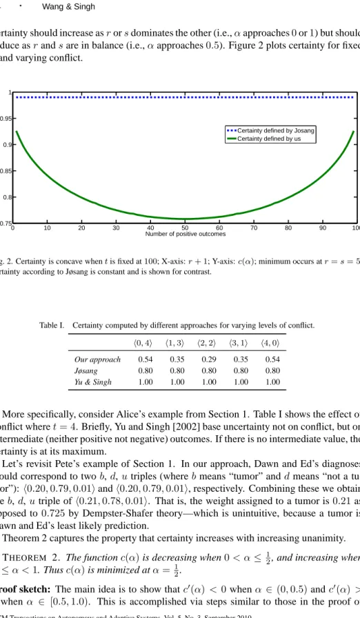
certainty should increase asrorsdominates the other (i.e.,αapproaches0or1) but should reduce asrandsare in balance (i.e.,αapproaches0.5). Figure 2 plots certainty for fixed tand varying conflict.
0 10 20 30 40 50 60 70 80 90 100 0.75 0.8 0.85 0.9 0.95 1
Number of positive outcomes
Certainty
Certainty defined by Josang Certainty defined by us
Fig. 2. Certainty is concave whentis fixed at100; X-axis:r+ 1; Y-axis:c(α); minimum occurs atr=s= 5; certainty according to Jøsang is constant and is shown for contrast.
Table I. Certainty computed by different approaches for varying levels of conflict. h0,4i h1,3i h2,2i h3,1i h4,0i
Our approach 0.54 0.35 0.29 0.35 0.54
Jøsang 0.80 0.80 0.80 0.80 0.80
Yu & Singh 1.00 1.00 1.00 1.00 1.00
More specifically, consider Alice’s example from Section 1. Table I shows the effect of conflict wheret= 4. Briefly, Yu and Singh [2002] base uncertainty not on conflict, but on intermediate (neither positive not negative) outcomes. If there is no intermediate value, the certainty is at its maximum.
Let’s revisit Pete’s example of Section 1. In our approach, Dawn and Ed’s diagnoses would correspond to twob,d,utriples (wherebmeans “tumor” anddmeans “not a tu-mor”):h0.20,0.79,0.01iandh0.20,0.79,0.01i, respectively. Combining these we obtain theb,d,utriple ofh0.21,0.78,0.01i. That is, the weight assigned to a tumor is0.21as opposed to0.725by Dempster-Shafer theory—which is unintuitive, because a tumor is Dawn and Ed’s least likely prediction.
Theorem 2 captures the property that certainty increases with increasing unanimity. THEOREM 2. The functionc(α)is decreasing when0< α≤ 12, and increasing when
1
2 ≤α <1. Thusc(α)is minimized atα= 1 2.
Proof sketch: The main idea is to show thatc′(α) < 0whenα∈ (0,0.5)andc′(α)> 0 when α ∈ [0.5,1.0). This is accomplished via steps similar to those in the proof of ACM Transactions on Autonomous and Adaptive Systems, Vol. 5, No. 3, September 2010.
Theorem 1. First remove the absolute sign, then differentiate, then prove the derivative is negative in the interval(0,0.5)and positive in the interval(0.5,1).
0 5 10 15 20 0 10 200 0.2 0.4 0.6 0.8 # of positive outcomes # of negative outcomes Certainty
Fig. 3. X-axis:r, number of positive outcomes; Y-axis:s, number of positive outcomes; Z-axis: certaintyc(r, s), the corresponding certainty.
Putting the above results together suggests that the relationship between certainty on the one hand and positive and negative evidence on the other hand is nontrivial. Figure 3 confirms this intuition by plotting certainty againstrandsas a surface. The surface rises on the left and right corresponding to increasing unanimity of negative and positive evi-dence, respectively, and falls in the middle as the positive and negative evidence approach parity. The surface trends upward going from front to back corresponding to the increasing evidence at a fixed level of conflict.
0 2 4 6 8 10 12 14 16 18 20 0.2 0.4 0.6 0.8 0.2 0.4 0.6
Total number of transactions
Certainty and conflict
Certainty
Conflict
Fig. 4. Certainty increases as unanimous evidence increases; the addition of conflicting evidence lowers certainty; X-axis: number of transactions. Y-axis:ccertainty.
It is worth emphasizing that certainty does not necessarily increase even as the evidence grows. When additional evidence conflicts with the previous evidence, a growth in evi-dence can possibly yield a loss in certainty. This accords with intuition because the arrival of conflicting evidence can shake one’s beliefs, thus lowering one’s certainty.
Figure 4 demonstrates a case where we first acquire negative evidence, thereby increas-ing certainty. Next we acquire positive evidence, which conflicts with the previous evi-dence, thereby lowering certainty. In Figure 4, the first ten transactions are all negative; the next ten transactions are all positive. Certainty grows monotonically with unanimous evidence and falls as we introduce conflicting evidence. Because of the dependence of certainty on the size of the total body of evidence, it does not fall as sharply as it rises, and levels off as additional evidence is accrued.
4.3 Bijection Between Evidence and Trust Reports
A major motivation for modeling trust and evidence spaces is that each space facilitates computations of different kinds. Discounting trust is simple in the trust space whereas aggregating trust is simple in the evidence space.
Recall that, as Theorem 1 shows, we associate greater certainty with larger bodies of evidence (assuming conflict is fixed). Thus the certainty of trust reports to be combined clearly matters: we should place additional credence where the certainty is higher (gener-ally meaning the underlying evidence is stronger). Consequently, we need a way to map a trust report to its corresponding evidence in such a manner that higher certainty yields a larger body of evidence. The ability to combine trust reports effectively relies on being able to map between the evidence and the trust spaces. With such a mapping in hand, to combine two trust reports, we would simply perform the following steps:
(1) Map trust reports to evidence. (2) Combine the evidence.
(3) Transform the combined evidence to a trust report.
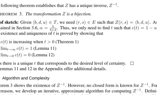
The following theorem establishes thatZhas a unique inverse,Z−1.
THEOREM 3. The transformationZis a bijection.
Proof sketch: Givenhb, d, ui ∈T, we need(r, s)∈Esuch thatZ(r, s) =hb, d, ui. As explained in Section 3.6,α= b
b+d. Thus, we only need to findtsuch thatc(t) = 1−u. The existence and uniqueness oftis proved by showing that
(1) c(t)is increasing whent >0(Theorem 1) (2) limt→∞c(t) = 1(Lemma 11)
(3) limt→0c(t) = 0(Lemma 12)
Thus there is a uniquetthat corresponds to the desired level of certainty. Lemmas 11 and 12 in the Appendix offer additional details.
4.4 Algorithm and Complexity
Theorem 3 shows the existence ofZ−1. However, no closed form is known forZ−1. For
this reason, we develop an iterative, approximate algorithm for computingZ−1.
Defini-tion 5, which provides the basis for DefiniDefini-tion 7, lies at the heart of our algorithm. We calculate the integral of Definition 5 via an application of the well-known trapezoidal rule. ACM Transactions on Autonomous and Adaptive Systems, Vol. 5, No. 3, September 2010.
To further improve performance, we cache a matrix of certainty values for different values of positive and negative evidence.
Notice thatαas b+bd. Furtherr =tαands =t(1−α). But we do not immediately knowt. In essence, no closed form forZ−1is known because no closed form is known for itstcomponent. The intuition behind our algorithm for computingtis that after fixingα, the correct value oftis one that would yield the desired certainty of(1−u). This works because, as remarked in the proof sketch for Theorem 3,c(t)ranges between0and1. Fur-ther, Theorem 1 shows that for fixedα,c(t)is monotonically increasing witht. In general, tbeing the size of the body of evidence is not bounded. However, as a practical matter, an upper bound can be placed ont. Thus, a binary search is an obvious approach. (When no bound is known, a simple approach would be to (1) guess exponentially increasing values fortuntil a value is found for which the desired certainty is exceeded; and then (2) conduct binary search between that and the previously guessed value.) Since we are dealing with real numbers, it is necessary to specifyǫ >0, the desired precision to which the answer is to be computed. (In our experiments, we setǫ= 10−4.)
Algorithm 1 calculatesZ−1via binary search onc(t)to a specified precision, ǫ > 0.
Heretmax >0is the maximum size of the body of evidence considered. (Recall thatlg means logarithm to base2.)
α=b+bd;c= 1−u;t1= 0;t2=tmax; whilet2−t1≥ǫdo t=t1+t2 2 ; ifc(t)< cthent1=t; elset2=t; end returnhtα, t(1−α)i Algorithm 1: Calculatinghr, si=Z−1(b, d, u).
THEOREM 4. The complexity of Algorithm 1 isΩ(−lgǫ).
Proof: After the while loop iteratesitimes,t2−t1 =tmax2−i. Eventually,t2−t1falls
below ǫ, thus terminating the loop. Assume the loop terminates inniterations. Then, t2 −t1 = tmax2−n < ǫ ≤ tmax2−n+1. This implies2n > tmaxǫ ≥ 2n−1. That is, n >(lgtmax−lgǫ)≥n−1.
4.5 Empirical Evaluation
The experimental validation of this work is made difficult by the lack of established datasets and testbeds, especially those that would support more than a scalar representation of trust. The situation is improving in this regard [Fullam et al. 2005], but current testbeds do not support exchanging trust reports of two dimensions (as inhb, d, uibecauseb+d+u= 1). We have evaluated this approach on two datasets. The first dataset includes ratings received by five sellers (of Slumdog Millionaire Soundtracks) on Amazon Marketplace. Amazon supports integer ratings from1 to5. Amazon summarizes the information on each seller as an average score along with the total number of ratings received. However, Amazon also makes the raw ratings available—these are what we use. We map the ratings to evidencehr, si, wherer+s= 1. Specifically, we map1toh0.0,1.0i,2toh0.25,0.75i, ACM Transactions on Autonomous and Adaptive Systems, Vol. 5, No. 3, September 2010.
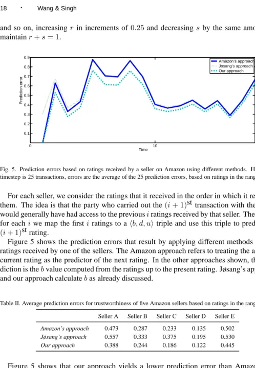
and so on, increasingr in increments of0.25and decreasing sby the same amount to maintainr+s= 1. 0 10 0.1 0.2 0.3 0.4 0.5 0.6 0.7 0.8 0.9 Time Prediction error Amazon’s approach Josang’s approach Our approach
Fig. 5. Prediction errors based on ratings received by a seller on Amazon using different methods. Here, one timestep is 25 transactions, errors are the average of the 25 prediction errors, based on ratings in the range [1, 5].
For each seller, we consider the ratings that it received in the order in which it received them. The idea is that the party who carried out the(i+ 1)st transaction with the seller would generally have had access to the previousiratings received by that seller. Therefore, for eachiwe map the firstiratings to ahb, d, uitriple and use this triple to predict the (i+ 1)st rating.
Figure 5 shows the prediction errors that result by applying different methods on the ratings received by one of the sellers. The Amazon approach refers to treating the average current rating as the predictor of the next rating. In the other approaches shown, the pre-diction is thebvalue computed from the ratings up to the present rating. Jøsang’s approach and our approach calculatebas already discussed.
Table II. Average prediction errors for trustworthiness of five Amazon sellers based on ratings in the range [1, 5]. Seller A Seller B Seller C Seller D Seller E
Amazon’s approach 0.473 0.287 0.233 0.135 0.502
Jøsang’s approach 0.557 0.333 0.375 0.195 0.530
Our approach 0.388 0.244 0.186 0.122 0.445
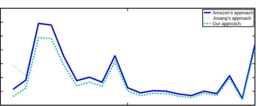
Figure 5 shows that our approach yields a lower prediction error than Amazon and Jøsang’s approaches. Jøsang’s approach is worse than Amazon’s whereas ours is better. The results for the other sellers are similar, and we omit them for brevity. Table II summa-rizes the results for all five sellers and shows that the same pattern holds for them.
We next evaluate our approach with respect to its ability to track a changing behavior pattern. To develop this test-case while staying in the realm of actual data, we artificially construct a seller whose ratings are a concatenation of the ratings obtained by different sell-ers. In this way, this seller models a seller who changes his behavior midstream (although, because all the sellers have high ratings, the change in behavior is not totally arbitrary). Figure 6 shows the results of applying the above approaches to this artificial seller. It finds ACM Transactions on Autonomous and Adaptive Systems, Vol. 5, No. 3, September 2010.
0 10 20 0.1 0.2 0.3 0.4 0.5 0.6 0.7 Time Prediction error Amazon’s approach Josang’s approach Our approach
Fig. 6. Prediction errors based on ratings received by an artificial “multiple personality” seller using different methods. This seller’s list of ratings is a concatenation of the ratings of the actual sellers. Here, one timestep is 50 transactions and shows the average prediction errors, based on ratings in the range [1, 5].
that the same pattern of results holds as in Figure 5. In Figure 6 too, Jøsang’s approach yields worse results than Amazon whereas our approach yields superior results. Notice, however, that data from marketplaces such as Amazon and eBay is inherently positive: partly it is because it is in the marketplace’s interest to promote higher ratings and partly it is because only sellers with high ratings survive to have many transactions.
A possible way to understand these results is the following. Amazon calculates the average rating as the prediction whereas Jøsang incorporates Laplace smoothing (recall the discussion in Section 3.2). Thus Jøsang ends up with higher error in many cases. Further, Jøsang’s definition of certainty ignore conflict and thus increases monotonically with evidence. Thus his predictions are the worst. Our approach takes a more nuanced approach than Amazon’s but without the pitfalls of Jøsang’s approach, and thus produces better results.
The second evaluation of the proposed approach is based on its use within trust propa-gation operators. Recently, Hang et al. [2009] proposed trust propapropa-gation operators based on the approach described in this paper. They evaluated their operators using two net-work datasets, namely, FilmTrust (538 vertices representing users; 1,234 weighted directed edges representing ratings) [Kuter and Golbeck 2007] and the PGP web of trust (39,246 vertices representing users (or rather keys) and 317,979 weighted directed edges repre-senting the strength of an endorsement) [WoT 2009]. Hang et al. report how the operators based on our approach perform better than other approaches applied on those datasets. We lack the space to fully describe their approach here.
5. LITERATURE
A huge amount of research has been conducted on trust. We now review some of the most relevant literature from our perspective of an evidential approach.
5.1 Literature on Distributed Trust
In general, the works on distributed trust emphasize techniques for propagating trust. In this sense, they are not closely related to the present approach, which emphasizes evidence and only indirectly considers propagation. Many of the existing approaches rely on sub-ACM Transactions on Autonomous and Adaptive Systems, Vol. 5, No. 3, September 2010.
jective assessments of trust. Potentially, one could develop variants of these propagation algorithms that apply on evidence-based trust reports instead of subjective assessments. However, two challenges would be (1) accommodatinghb, d, uitriples instead of scalars; and (2) conceptually making sense of the propagated results in terms of evidence. Hang et al. [2009], discussed above, address both of these challenges.
Carbone et al. [2003] propose a two-dimensional representation of trust consisting of (1) trustworthiness and (2) certainty placed in the trustworthiness. Their proposal is abstract and lacks a probabilistic interpretation; they do not specify how to calculate certainty or any properties of it. Carbone et al. do not discuss how the trust originates or relates with evidence. The level of trustworthiness for them is the extent to which, e.g., the amount of money loaned, an agent will fully trust another. Weeks [2001] introduces a mathe-matical framework for distributed trust management. He defines the semantics of trust computations as the least fixed point in a lattice. Importantly, Weeks only deals with the so-called hard trust among agents that underlies traditional authorization and access control approaches. He does not deal with evidential trust, as studied in this paper.
Several approaches understand trust in terms of aggregate properties of graphs, such as can be described via matrix operations [Guha et al. 2004]. The propagation of trust corresponds to matrix multiplication. Such aggregate methods can be attractive and have a history of success when applied to link analysis of web pages. Such link analysis is inspired by the random browser model. However, it is not immediately apparent why trust should map to the random browser model, or whether it is even fair to expect trust ratings to be public the way links on web pages are. A further unintuitive consequence is that to ensure convergence these approaches split trustworthiness. For example, if Alice trusts two people but Bob only trusts only one person, Alice’s trustworthiness is split between two people but Bob’s trustworthiness propagates fully to his sole contact. There is no conceptual reason for this discrepancy.
Ziegler and Lausen [2004] model trust as energy to be propagated through spreading activation. They treat trust as a subjective rating based on opinions, not evidence. They do not justify the energy interpretation conceptually. Ziegler and Lausen’s notion of trust is global in that each party ends up with an energy level that describes its trustworthiness. Thus the relational aspect of trust is lost. The above remark about splitting trustworthiness among multiple parties applies to energy based models as well.
Quercia et al. [2007] relate nodes (corresponding to mobile users) based on the similarity of their ratings, and apply a graph-based learning technique by which a node may compute its rating of another node. Their method is similar to collaborative filtering applied by each node. Crucially, Quercia et al.’s model is based on subjective ratings, not evidence. However, our approach could potentially be combined with the prediction part of Quercia et al.’s model. Kuter and Golbeck [2007] propagate trust by combining trust ratings across all paths from a source to a sink vertex in a graph, along with a confidence measure. The underlying data are subjective ratings, not evidence.
Schweitzer et al. [2006] apply Jøsang’s representation in ad hoc networks. Their ap-proach is heuristic and does not explicitly accommodate certainty, unlike Hang et al. [2009]. Schweitzer et al. enable a participant to withdraw its previous recommendations of another party.
5.2 Literature on Trust and Evidence
Abdul-Rahman and Hailes [2000] present an early, ad hoc model for computing trust. Specifically, various weights are simply added up without any mathematical justification. Likewise, the term uncertainty is described but without any mathematical foundation.
Sierra and Debenham [2007] define an agent strategy by combining the three dimensions of utility, information, and semantic views. They justify their, rather complex, framework based on intuitions and experimental evaluations. Thus it is conceptually plausible, but lacks an explicit mathematical justification, such as in the present approach.
The Regret system combines several aspects of trust, notably the social aspects [Sabater and Sierra 2002]. It involves a number of formulas, which are given intuitive, but not math-ematical, justification. A lot of other work, e.g., [Huynh et al. 2006], involves heuristics that combine multiple information sources to judge trust. It would be an interesting direc-tion to combine a rigorous approach such as ours with the above heuristic approaches to capture a rich variety of practical criteria well.
Teacy et al. [2005] propose TRAVOS, the Trust and Reputation model for Agent-based Virtual OrganisationS, which uses a probabilistic treatment of trust. They model trust in terms of confidence that the expected value lies within a specified error tolerance. They study combinations of probability distributions corresponding to evaluations given by dif-ferent agents, but do not formalize certainty. Further, Teacy et al.’s approach does not yield a probabilistically valid method for combining trust reports, as supported by our approach. Despotovic and Aberer [2005] propose maximum likelihood estimation to aggregate rat-ings, which admits a clear statistical interpretation and reduces the calculation overhead of propagating and aggregating trust information. However, their model is overly simplified, and requires binary rather than real valued ratings. Further, Despotovic and Aberer ignore the uncertainty of a rating. To estimate the maximum likelihood, each agent needs to record the trustworthiness of all possible witnesses, thus increasing the complexity. Further, since each agent only knows a small fraction of all agents, it often cannot compute how much trust to place in the necessary witnesses.
Reece et al. [2007] consolidate an agent’s direct experience with a provider and trust re-ports about that provider received from others. They calculate a covariance matrix based on the Dirichlet distribution that describes the uncertainty and correlations between different dimensional probabilities. This matrix can be used to communicate and fuse ratings. The Dirichlet distribution considers the ratio of positive and negative, but not the total number of, transactions. The resulting certainty estimates are independent of the total number of transactions, unlike in our approach. Lastly, Reece et al. neglect the trustworthiness of the agent who provides the information. in contrast with Wang and Singh [2006].
Halpern and Pucella [2006] treat evidence as an operator that maps prior to posterior beliefs. Like our certainty function, their confirmation function measures the strength of the evidence. However, many confirmation functions are available, and it is not clear which one to use. Halpern and Pucella use the log-likelihood ratio, not based on its optimality, but because it avoids requiring a prior distribution on hypotheses.
Fullam and Barber [2006] support decisions based on agent role (trustee or truster) and transaction type (fundamental or reputation). They apply Q-learning and explain why the learning is complicated for reputation. Fullam and Barber [2007] study different sources of trust information: direct experience, referrals from peers, and reports from third parties. They propose a dynamical learning technique to identify the best sources of trust. The ACM Transactions on Autonomous and Adaptive Systems, Vol. 5, No. 3, September 2010.
above works disregard uncertainty and do not offer mathematical justifications.
Li et al. [2008] describe ROSSE, a search engine for grid service discovery and matching based on rough set theory. They define a property as being uncertain when it is used in some but not all advertisements for services in the same category. Here, uncertainty means how unlikely a service is to have the property. This is quite different from our meaning based on outcomes.
Jurca and Faltings [2007] describe a mechanism that uses side payments as incentives for agents to truthfully report ratings of others. They ignore uncertainty, thus ignoring the strength of evidence. Overall, though, our approaches are complementary: they obtain in-dividual ratings; we aggregate the ratings into measures of certainty. Sen and Sajja [2002] also address deception, modeling agents as following either a low or a high distribution of quality. They estimate the number of raters (some liars) to query to obtain a desired likelihood of quality of a service provider, and study thresholds beyond which the number of liars can disrupt a system. Yu and Singh [2003] show how agents may adaptively detect deceptive agents. Yolum and Singh [2003] study the emergent graph-theoretic properties of referral systems. This paper complements such works because it provides an analytical treatment of trust that they do not provide whereas they address system concerns that this paper does not study.
5.3 Literature on Information Theory
Shannon entropy [1948] is the best known information-theoretic measure of uncertainty. It is based on a discrete probability distributionp=hp(x)|x∈Xiover a finite setX of al-ternatives (elementary events). Shannon’s formula encodes the number of bits required to obtain certainty:S(p) =−P
x∈Xp(x) lgp(x). HereS(p)can be viewed as the weighted average of the conflict among the evidential claims expressed byp. Jaynes [2003] provides examples, intuitions, and precise mathematical treatment of entropy. More complex, but less well-established, definitions of entropy have been proposed for continuous distribu-tions as well, e.g., [Smith 2001]. Entropy, however, is not suitable for the present purposes of modeling evidential trust. Entropy captures (bits of) missing information and ranges from0to∞. At one level, this disagrees with our intuition that, for the purposes of trust, we need to model the confidence placed in a probability estimation. Moreover, the above definitions cannot be used in measuring the uncertainty of the probability estimation based on past positive and negative experiences.
6. DISCUSSION
This paper contributes to a mathematical understanding of trust, especially as it underlies a variety of multiagent applications, especially in social networks and service-oriented computing. These include social networks understood via referral systems and webs of trust, in studying which we identified the need for this research. Such applications require a natural treatment of composition and discounting in an evidence-based framework.
An evidence-based notion of trust must accommodate the effects of increasing evidence (for constant conflict) and of increasing conflict (for constant evidence). Theoretical val-idation, as provided here, is valuable for a general-purpose mathematical approach. The main technical insight of this paper is how to manage the duality of trust and evidence spaces in a manner that provides a rigorous basis for combining trust reports. A benefit is that an agent who wishes to achieve a specific level of certainty can compute how much ev-idence would be needed at different levels of conflict. Or, the agent can iteratively compute ACM Transactions on Autonomous and Adaptive Systems, Vol. 5, No. 3, September 2010.