Application of Triangular Functions to Numerical
Solution of Stochastic Volterra Integral Equations
M. Khodabin
1, K. Maleknejad
2, F. Hosseini Shekarabi
3.
∗Abstract—In this paper, an efficient method for solving numerically stochastic Volterra integral equa-tion is proposed. Here, we consider triangular func-tions and their operational matrix of integration. This method has several advantages in reducing computa-tional burden and is more accurate than the BPFs. An error analysis is valid under fairly restrictive con-ditions. The method is applied to examples to illus-trate the accuracy and implementation of the method.
Keywords: Triangular functions; Operational Matrix; Stochastic operational matrix; Stochastic Volterra in-tegral equations; Itˆo integral.
1
Introduction
Wide variety of problems in physics, mechanics, economics, sociology, biological lead to the Stochastic Volterra Integral Equations (SVIEs). These systems are dependent on a noise source, on a Gaussian white noise, so modeling such phenomena naturally requires the use of various stochastic Volterra integral equations.
Most SVIEs can not be solved analytically and hence it is of great importance to provide numerical solution. So, there has been a growing interest in numerical solutions of stochastic Volterra integral equations for the last years [1,7,14,15,17,18].
In the present work, we consider
u(t) =u0(t) +
t
0 k1(s, t)u(s)ds+
t
0 k2(s, t)u(s)dB(s),
(1)
t∈[0, T),
where, u(t), u0(t),k1(s, t) and k2(s, t), for s, t ∈[0, T), are the stochastic processes defined on the same proba-bility space (Ω,F, P) with a filtration {Ft, t ≥ 0} that is increasing and right continuous andF0contains all
P-null sets. u(t) is unknown random function andB(t) is a standard Brownian motion defined on the probability space and0tk2(s, t)u(s)dB(s) is the Itˆo integral.
Triangular Functions (TFs) have been introduced by Deb
∗Department of Mathematics, Karaj Branch, Islamic Azad
Uni-versity, Karaj, Iran/1Corresponding Author. E-mail Address: [email protected] &2E-mail Address: [email protected]&
3E-mail Address: f [email protected].
et al. (2006) in [8], and TF approximation were success-fully applied for analysis of dynamic systems [8], vari-ational problems [6], integral equations [3,5], integro-differential equations [4], Nonlinear Constrained Opti-mal Control Problems [9], and Volterra-Fredholm integral equations [2,12,13].
This paper is organized as follows: In the next section we review one-dimensional triangular functions. Section 3, presents stochastic concept that is used in this paper. Section 4, introduces stochastic integration operational matrix related to TFs. In Section 5, TF method is applied to solve stochastic Volterra integral equations. Section 6, investigates error analysis of method. In Section 7, numerical results are shown. Finally, Section 8, provides the conclusion.
2
Triangular functions(TFs)
In this section definitions of the TFs and their prop-erties are reviewed. Two m-sets of triangular functions are defined over the interval [0, T) as
Ti1(t) =
1−t−hih ih≤t <(i+ 1))h,
0 elsewhere. (2)
Ti2(t) = t−ih
h ih≤t <(i+ 1))h,
0 elsewhere. (3)
where, i= 0, ..., m−1. mis the number of elementary functions and h= T
m. In this paper, it is assumed that
T = 1, so, TFs are defined over [0,1), andh= m1. More-over,
Ti1(t) +Ti2(t) =φi(t), (4) where, φi(t) is theith block pulse function:
φi(t) =
1 (i)h≤t <(i+ 1)h,
0 elsewhere. (5)
From the definition of TFs, it is clear that TFs are dis-joint, orthogonal, and complete [8]. Therefore it can be written
1
0 T
p
i(t)Tjq(t)dt=δijp,q, (6)
IAENG International Journal of Applied Mathematics, 43:1, IJAM_43_1_01
where,δij is Kronecker delta and
p,q= h
3 p=q∈ {1,2},
h
6 p=q.
(7)
The set of TFs may be written as a vector T1(t) and
T2(t) of dimensionm
T1(t) = [T01(t), ..., Tm1−1(t)]T,
T2(t) = [T02(t), ..., Tm2−1(t)]T, (8) and
T(t) = [T1(t), T2(t)]T, (9) where,T(t) is called the 1D-TF vector.
From the above representation and disjointness property, it follows:
T(t).TT(t)diag(T(t)) =T(t), (10) where,Tis a 2m×2mdiagonal matrix.
The expansion of a functionf(t) over [0, T) with respect to 1D-TFs,i= 0, ..., m−1 is given by
f(t) m−1
i=0
C1iTi1(t) + m−1
i=0
C2iTi2(t)
=C1T.T1(t) +C2T.T2(t)
= [C1, C2]T.[T1(t), T2(t)] =CT.T(t), (11) where,C1iandC2iare samples off, for exampleC1i=
f(ih) andC2i=f((i+ 1)h) fori= 0,1, .., m−1,and as a result there is no need for integration. The vectorC is called the 1D-TF coefficient vector.
Now, integration operational matrix of TFs is considered t
0 T1(s)ds=P1.T1(t) +P2.T2(t), (12)
t
0 T2(s)ds=P1.T1(t) +P2.T2(t), (13)
where,
P1 = h 2
⎛ ⎜ ⎜ ⎜ ⎜ ⎜ ⎝
0 1 1 . . . 1 0 0 1 . . . 1 0 0 0 . . . 1 ..
. ... ... . .. ... 0 0 0 . . . 0
⎞ ⎟ ⎟ ⎟ ⎟ ⎟ ⎠
m×m
, (14)
P2 = h 2
⎛ ⎜ ⎜ ⎜ ⎜ ⎜ ⎝
1 1 1 . . . 1 0 1 1 . . . 1 0 0 1 . . . 1 ..
. ... ... . .. ... 0 0 0 . . . 1
⎞ ⎟ ⎟ ⎟ ⎟ ⎟ ⎠
m×m
. (15)
Therefore, t
0
T(s)dsP.T(t), (16) where,Pis operational matrix of integration that is given by
P =
P1 P2
P1 P2
. (17)
So, we can approximate the integral of every function as t
0 f(s)ds
t
0 C
T.T(s)dsCT.P.T(t). (18)
Assuming that k(s, t) is a function of two variables. It can be expanded with respect to TFs as follows
k(s, t) =TT(t)KT(s), (19) where, T(s) and T(t) are 2m1-dimensional and 2m2 -dimensional triangular vectors and K is a 2m1 ×2m2
coefficient matrix of TFs. For convenience, we put m1=
m2=m.So, matrix K can be written as
K =
K11 K12
K21 K22
, (20)
where, K11, K12, K21, and K22 can be computed by sampling the functionk(s, t) at pointssiandtisuch that
si=ti=ih,fori= 0,1, ..., m.Therefore
(K11)i,j =k(si, tj);i= 0,1, ..., m−1, j = 0,1, ..., m−1,
(K12)i,j =k(si, tj);i= 0,1, ..., m−1, j= 1, ..., m, (K21)i,j =k(si, tj);i= 1, ..., m, j= 0,1, ..., m−1,
(K22)i,j=k(si, tj);i= 1, ..., m, j= 1, ..., m.
Now, let B be a 2m×2mmatrix. So, it can be similarly concluded that
TT(t)BT(t)BT (t), (21) in which, B is a 2m-vector with elements equal to the diagonal entries of matrixB.Furthermore,
T(t)TT(t)XXT˜ (t),
where, ˜X = diag(X) is 2m×2mdiagonal matrix. The following integral can be computed
1
0
T(t)TT(t)dtD, (22)
where, Dis the following 2m×2mmatrix
D= h
3Im×m h6Im×m h
6Im×m h3Im×m
. (23)
IAENG International Journal of Applied Mathematics, 43:1, IJAM_43_1_01
3
Stochastic concepts and Ito integral
Definition 3.1. (Brownian motion process). Brownian motion B(t) is a stochastic process with the following properties.
(i) (Independence of increments)B(t)−B(s), fort > s,
is independent of the past.
(ii) (Normal increments)B(t)−B(s) has Normal distribu-tion with mean 0 and variancet−s.This implies (taking s = 0) thatB(t)−B(0) hasN(0, t) distribution. (iii) (Continuity of paths)B(t), t≥0 are continuous func-tions oft.
Definition 3.2. Let {N(t)}t≥0 be an increasing family
of σ-algebras of sub-sets of Ω. A process g(t, ω) from [0,∞)×Ω toRn is calledN(t)-adapted if for eacht≥0 the functionω−→g(t, ω) isN(t)-measurable [16].
Definition 3.3. Letν=ν(S, T) be the class of functions
f(t, ω) : [0,∞)×Ω−→Rsuch that,
(i) (t, ω)−→ f(t, ω), is B× F-measurable, whereB de-notes the Borelσ-algebra on [0,∞) andF is theσ-algebra on Ω.
(ii) f(t, ω) isFt-adapted, whereFt is theσ-algebra gen-erated by the random variablesB(s);s≤t.
(iii) E STf2(t, ω)dt]<∞.
Proof. see [16]
Definition 3.4. (The Itˆo integral), [16]. Letf ∈ν(S, T), then the Itˆo integral off (from S to T) is defined by
T
S
f(t, ω)dB(t)(ω) = lim n→∞
T
S
φn(t, ω)dB(t)(ω),
(limit in L2(P))
where,φnis a sequence of elementary functions such that
E
T
S
(f(t, ω)−φn(t, ω))2dt→0, as n→ ∞.
Theorem 3.5. (The Itˆo isometry). Let f ∈ ν(S, T), then
E( T
S
f(t, ω)dB(t)(ω))2=E
T
S
f2(t, ω)dt.
Proof. [16]
Definition 3.6. (1-dimensional Itˆo processes), [16]. Let
B(t) be 1-dimensional Brownian motion on (Ω,F, P). A 1-dimensional Itˆo process (stochastic integral) is a stochastic processX(t) on (Ω,F, P) of the form
X(t) =X(0) + t
0 u(s, ω)ds+
t
0 v(s, ω)dB(s),
or
dX(t) =udt+vdB(t), (24) where
P
t
0
v2(s, ω)ds <∞, f or all t≥0= 1,
P
t
0 |
u(s, ω)|ds <∞, f or all t≥0= 1.
Theorem 3.7. (The 1-dimensional Itˆo formula). Let
X(t) be an Itˆo process given by (1) and g(t, x) ∈
C2([0,∞)×R), then
Y(t) =gt, X(t),
is again an Itˆo process, and
dY(t)
= ∂g
∂t
t, X(t)dt+∂g
∂x
t, X(t)dX(t)+1 2
∂2g ∂x2
t, X(t)dX(t)2,
(25) where (dX(t))2 = (dX(t))(dX(t)) is computed according to the rules,
dt.dt=dt.dB(t) =dB(t).dt= 0, dB(t).dB(t) =dt.
(26)
Proof. see [16].
Furthermore, we will apply several times the usual ele-mentary equalities
( m
i=1
ai)r≤mr−1 m
i=1
ari, ai>0, r∈N, (27)
and
|a+b|r≤(2r−1∨1)(|a|r+|b|r), r≥0. (28) Also.is notation of
f(t)2= 1
0 |f(t)| 2dt.
Lemma 3.8. (The Gronwall inequality) Let α, β ∈
[t0, T]→Rbe integral with
0≤α(t)≤β(t) +L
t
t0
α(s)ds.
for t∈[t0, T] where,L >0. Then
α(t)≤β(t) +L
t
t0
eL(t−s)β(s)ds, t∈[t
0, T].
For more details see [10,11,16,19].
IAENG International Journal of Applied Mathematics, 43:1, IJAM_43_1_01
4
Stochastic integral operational matrix
for triangular functions
The Ito integral of eachTi1 andTi2is defined by t
0
Ti1(s)dB(s)
= ⎧ ⎪ ⎪ ⎪ ⎪ ⎪ ⎪ ⎪ ⎪ ⎪ ⎪ ⎪ ⎪ ⎪ ⎪ ⎪ ⎪ ⎨ ⎪ ⎪ ⎪ ⎪ ⎪ ⎪ ⎪ ⎪ ⎪ ⎪ ⎪ ⎪ ⎪ ⎪ ⎪ ⎪ ⎩ 0
0≤t < ih,
(i+ 1)[B(t)−B(ih)]−iht s hdB(s)
ih≤t <(i+ 1)h,
(i+ 1)[B((i+ 1)h)−B(ih)]−ih(i+1)hshdB(s) (i+ 1)h≤t < T,
(29) fori= 0, ..., m−1.
t
0 T 2
i(s)dB(s)
= ⎧ ⎪ ⎪ ⎪ ⎪ ⎪ ⎪ ⎪ ⎪ ⎪ ⎪ ⎪ ⎪ ⎪ ⎪ ⎪ ⎪ ⎨ ⎪ ⎪ ⎪ ⎪ ⎪ ⎪ ⎪ ⎪ ⎪ ⎪ ⎪ ⎪ ⎪ ⎪ ⎪ ⎪ ⎩ 0
0≤t < ih,
−i[B((t)−B(ih)] +iht shdB(s)
ih≤t <(i+ 1)h,
−i[B((i+ 1)h)−B(ih)] +ih(i+1)h s hdB(s) (i+ 1)h≤t < T,
(30)
fori= 0, ..., m−1.
We approximate B(t) − B(ih), by B((i + 0.5)h) −
B(ih), at mid-point of [ih,(i+ 1)h)]. Also, iht hsdB(s) with ih(i+0.5)hs
hdB(s). As a result, t
0Ti1(s)dB(s), and t
0Ti2(s)dB(s) with 1D-TF are taken in the vector form
as
t
0 T 1
i(s)dB(s) [0,0, . . . ,0,
(i+ 1)[B((i+ 0.5)h)−B(ih)]−
(i+0.5)h
ih
s hdB(s),
(i+ 1)[B((i+ 1)h)−B(ih)]−
(i+1)h
ih
s
hdB(s), . . . ,
(i+ 1)[B((i+ 1)h)−B(ih)]−
(i+1)h s
hdB(s)](T1 +T2),
in which the ith component is (i+ 1)[B((i+ 0.5)h)−
B(ih)]−ih(i+0.5)hs
hdB(s) and t
0 T 2
i(s)dB(s)
[0,0, . . . ,0,−i[B((i+0.5)h)−B(ih)]+
(i+0.5)h
ih
s hdB(s),
−i[B((i+ 1)h)−B(ih)] +
(i+1)h
ih
s
hdB(s), . . . ,
−i[B((i+ 1)h)−B(ih)] +
(i+1)h
ih
s
hdB(s)](T1 +T2).
Considering following definitions,
α(i) := (i+ 1)[B((i+ 0.5)h)−B(ih)]−
(i+0.5)h
ih
s hdB(s),
β(i) := (i+ 1)[B((i+ 1)h)−B(ih)]−
(i+1)h
ih
s hdB(s),
γ(i) :=−i[B((i+ 0.5)h)−B(ih)] +
(i+0.5)h
ih
s hdB(s),
ρ(i) :=−i[B((i+ 1)h)−B(ih)] +
(i+1)h
ih
s hdB(s),
stochastic operational matrix of integration is given by
P1S= ⎛ ⎜ ⎜ ⎜ ⎜ ⎜ ⎜ ⎜ ⎜ ⎜ ⎜ ⎜ ⎜ ⎜ ⎜ ⎜ ⎝
α(0) β(0) β(0) . . . β(0)
0 α(1) β(1) . . . β(1)
0 0 α(2) . . . β(2)
..
. ... ... ... ...
0 0 0 . . . β(m−2)
0 0 0 . . . α(m−1) ⎞ ⎟ ⎟ ⎟ ⎟ ⎟ ⎟ ⎟ ⎟ ⎟ ⎟ ⎟ ⎟ ⎟ ⎟ ⎟ ⎠
m×m
, (31)
P2S= ⎛ ⎜ ⎜ ⎜ ⎜ ⎜ ⎜ ⎜ ⎜ ⎜ ⎜ ⎜ ⎜ ⎜ ⎜ ⎜ ⎝
γ(0) ρ(0) ρ(0) . . . ρ(0)
0 γ(1) ρ(1) . . . ρ(1)
0 0 γ(2) . . . ρ(2)
..
. ... ... ... ...
0 0 0 . . . ρ(m−2)
0 0 0 . . . γ(m−1) ⎞ ⎟ ⎟ ⎟ ⎟ ⎟ ⎟ ⎟ ⎟ ⎟ ⎟ ⎟ ⎟ ⎟ ⎟ ⎟ ⎠
m×m
, (32)
t
0 T1(s)dB(s) =P1s.T1(t) +P1s.T2(t), (33)
IAENG International Journal of Applied Mathematics, 43:1, IJAM_43_1_01
t
0
T2(s)dB(s) =P2S.T1(t) +P2S.T2(t). (34) Therefore
t
0
T(s)dB(s)PS(T1 +T2) =PS.T(t), (35) where, PS the stochastic operational matrix of integra-tion in the 1D-TF domain, can be represent as
PS=
P1S P1S
P2S P2S
. (36)
So, the Itˆo integral of every functionf(t) can be approx-imated as follows
t
0 f(s)dB(s)
t
0 C
TT(s)dB(s)CTP
ST(t). (37) .
5
Application of TFs to solve SVIEs
Here this method is applied for Eq.(1)
u(t) =u0(t) + t
0
k1(s, t)u(s)ds+ t
0
k2(s, t)u(s)dB(s)
t∈[0, T],
we approximate function u(t), u0(t), k1(s, t), k2(s, t) by
TFs,
u(t)u¯(t) =UTT(t) =TT(t)U, (38)
u0(t)U0TT(t) =TT(t)U0, (39)
k1(s, t)TT(t)K1T(s), (40)
k2(s, t)TT(t)K
2T(s), (41)
where, the vectors U, U0, and matrices K1, K2 are TFs coefficient of u, u0, k1 andk2 respectively.
Substituting (38-41) into (1), we get
TT(t)UTT(t)U0+
t
0 T
T(t)K
1T(s)TT(s)U ds+
t
0 T(t)
TK
2T(s)TT(s)U dB(s).
Using previous relations
TT(t)UTT(t)U0+TT(t)K1
t
0 T(s)T
T(s)U ds+
TT(t)K2
t
0 T(s)T
T(s)dB(s)
=TT(t)U
0+TT(t)K1U P T (t) +TT(t)K2U P ST(t), (42) where, U = diag(U), K1U P and K2U P S are 2m×2m matrices. Eq.(21) gives
TT(t)K1U P T (t)B1TT(t) =TT(t)B1,
TT(t)K
2U P ST(t)B2TT(t) =TT(t)B2T,
in which, B1 and B2 are 2m-vectors with components equal to the diagonal entries of the matrices K1U P ,
K2U P S respectively. B1,B2can be written as
B1= ΠU,
B2= ΠSU,
where, Π and ΠS are 2m×2mmatrices with components Πi,j = (K1)i,jPj,i, i, j= 1...m,
(ΠS)i,j = (K2)i,j(PS)j,i, i, j = 1...m.
Then,
TT(t)U TT(t)U0+TT(t)Π.U+TT(t)ΠS.U, by replacingwith =,it gives
(I−Π−Πs)U =U0. (43) After solving the linear system (43) U is calculated and as a resultu(t) of (38) is approximated.
6
Error analysis
In following theorems for simplicity we assumeT = 1 and h= m1. Moreover
f(x)fm(x) = m−1
i=0
C1iT1i(x) +C2iT2i(x)
= [f(0), f(h), ..., f((m−1)h)]T1+[f(h), f(2h), ..., f(mh)]T2 =C1TT1 +C2TT2. (44)
Theorem 6.1. Assume that:
(1)f(x)is continuous on[0,1]and twice differentiable in (0,1),
(2)fm(x)are correspondingly to TFs, (3) |f(x)|< M for every x∈[0,1].
Then
f(x)−fm(x)=O(h2).
IAENG International Journal of Applied Mathematics, 43:1, IJAM_43_1_01
Proof: Suppose ti = mi = ih and Ii = [ti, ti+1]. The
representation error when f(x) is represented in a series of TFs over every subinterval [ti, ti+1],i= 0, ..., m−1 is
ei(x) =f(x)−C1TiT1i(x)−C2TiT2i(x), where
C1i=f(ih), C2i=f((i+ 1)h).
Base on Taylor’s series, the error forf(x) =C(constant) andf(x) =x,f(x) =x2 are computed.
It is obvious thatf(x) =C;ei(x) = 0.
So, this error for f(x) = x in interval [ti, ti+1], is computed by
ei(x)[ti,ti+1]=|x−C1iT1−C2iT2|
=|x−[ih(1−(x−ih)
h )−((i+ 1)h)
(x−ih)
h ]|= 0.
Then the error forf(x) =x2is
ei(x)[ti,ti+1]
=|x2−[(ih)2(1− (x−ih)
h )−((i+ 1)h)
2(x−ih)
h ]|
=|x2+i2h2−2hxi−hx+ih2|
≤ h2 4.
So, the error with TFs ish2M, x∈[ih,(i+ 1)h].
ei(x)2= ti+1
ti
|ei(x)|2dx= ti+1
ti
h4M2dx=M2h5,
e2
= 1
0
e2(x)dx= 1
0
( m−1
i=0
ei(x))2dx= m−1
i=0
1
0
e2i(x)dx
= m−1
i=0
ei2=m.M2h5=M2h4.
Hence,
f(x)−fm(x)=O(h2).
Now we assume thatf(x, y) is a twice differentiable func-tion on D = [0,1)×[0,1) such that second partial dif-ferential is bounded. We define the error between f(x,y) and its 2D-TFs expansion,fi,j,over every subregionDij,
as follows:
eij(x, y) =f(x, y)−fij.
where,
Dij :={(x, y)|ti≤x≤ti+1, tj≤x≤tj+1}.
For f(x, y) = C(constant), this error is zero, and also, for f(x, y) =ax+by, a, b∈R.
Now, we compute the error for
f(x, y) =ax2+by2+Cxy.
Using previous relation, error for f(x, y) = x2 and
f(x, y) =y2areM h2. Then error forf(x, y) =xy is
|xy−(ih(1−(x−ih)
h )+((i+1)h)
(x−ih)
h )(jh(1−
(y−jh)
h )+
((j+ 1)h)(y−jh)
h )|= 0.
This leads
eij(x, y)2= ti+1
ti
tj+1
tj
|ei,j(x, y)|2dydx
= ti+1
ti
tj+1
tj
h4M2dydx=M2h6.
e(x, y)2= 1
0
1
0 e
2(x, y)dydx
= 1
0
1
0 (
m−1
i=0
m−1
j=0
eij(x, y))2dydx
= 1
0
1
0
( m−1
i=0 m−1
j=0
e2ij(x, y))dydx+
2 i<i1
j<j1
1
0
1
0
ei,j(x, y)ei1,j1(x, y)dydx.
Since for i < i1,j < j1, we have
Di,j∩Di1,j1={},
then
e(x, y)2= m−1
i=0
m−1
j=0
1
0
1
0
e2ij(x, y))dydx
= m−1
i=0
m−1
j=0
eij2≤m2M2h6=M2h4.
Hence,
e(x, y)2=O(h2),
where, e(x, y) =fm(x, y)−f(x, y).
Theorem 6.2. Letu(t)andu¯(t)be solution of equation (1) and (38), respectively, and assume
1.u(t)< C.
2.ki< C i= 1,2. Then
sup0≤t≤T(E((u(t)−u¯(t)))2)1/2=O(h2), t∈[0,1].
IAENG International Journal of Applied Mathematics, 43:1, IJAM_43_1_01
Table 1: Mean, standard deviation and confidence interval for error mean in Example 1 with m=8.
n xE sE %95 confidence interval for mean of E
Lower U pper
30 0.0037718893 0.0027234708 0.0027973078 0.0047464708 50 0.0036791366 0.0019663909 0.0031340808 0.0042241924 100 0.0037348421 0.0024004921 0.0032643456 0.0042053386 200 0.0038060617 0.0020049289 0.0035281927 0.0040839307 500 0.0036943720 0.0021958184 0.0035019000 0.0038868440 1000 0.0037556983 0.0022554441 0.0036159044 0.0038954922
Table 2: Mean, standard deviation and confidence interval for error mean in Example 1 with m=16.
n xE sE %95 confidence interval for mean of E
Lower U pper
30 0.0030521307 0.0018854114 0.0023774449 0.0037268165 50 0.0032942542 0.0019295053 0.0027594226 0.0038290858 100 0.0030189793 0.0023418020 0.0025599861 0.0034779725 200 0.0030228432 0.0020486679 0.0027389123 0.0033067741 500 0.0032408144 0.0023818067 0.0030320398 0.0034495890
Proof: We have
u(t)−u¯(t) =u0(t)−u¯0(t)+ t
0 k1(s, t)u(s)−
¯
k1(s, t)¯u(s)ds+
t
0 k2(s, t)u(s)−
¯
k2(s, t)¯u(s)dB(s).
So,
E(u−u¯2)≤
3[E((u0−u¯0)2) +E( t
0
(k1u−k¯1u¯)ds2)
+E( t
0 (k2u−
¯
k2u¯)dB(s)2)] (45)
≤3[E((u0−u0)2) + (
t
0 E(k1u−k1u 2)ds)+
( t
0
E(k2u−k2u)2)ds],
by the Cauchy-Schwartz inequality and the linearity of Ito integrals in their integrands.
The first term satisfies by last theorem,
E(u0−u0)2)≤E(C2h4) =O(h4),
now,
(ki(s, t)u(t)−ki(s, t)u(t)2≤ 2(ki−ki)u2+2ki(u−u)2≤
C.(ki−ki2) +C.((u−u)2), i= 1,2,
furthermore,
ki−ki2=O(h4) i= 1,2. Hence
E(u−u2)≤ 3[E((u0−u0)2) +
t
0
E((k1u−k1u)2ds)+ t
0
E((k2u−k2u)2)ds]≤
CE(u0−u02) +C
t
0 E(k1−k1 2)ds+
C
t
0 E(k2−k2
2)ds+C t
0 E((u−u) 2)ds,
then by Gronwall’s inequality, we get
E((u−u)2))≤Ch4.
7
Numerical examples
In this section, the theoretical results of the previous sections are used for numerical examples. Let Xidenote the triangular coefficient of exact solution of the given example, andYibe the triangular coefficient of computed solution by the presented method. In these examples error is taken as
E∞= max1≤
i≤m|Xi−Yi|.
Example 1. Consider the following linear stochastic Volterra integral equation,
u(t) =1 3+
t
0 ln(s+1)u(s)ds+
t
0
ln(s+ 1)u(s)dB(s),
IAENG International Journal of Applied Mathematics, 43:1, IJAM_43_1_01
Table 3: Mean, standard deviation and confidence interval for error mean in Example 2 with m=8.
n xE sE %95 confidence interval for mean of E
Lower U pper
30 0.0071270253 0.0009796141 0.0067764748 0.0074775757 50 0.0070807614 0.0009460076 0.0068185414 0.0073429813 100 0.0071393177 0.0007080540 0.0070005391 0.0072780962 200 0.0071454450 0.0008471962 0.0070280295 0.0072628604 500 0.0070885786 0.0007660474 0.0070214315 0.0071557256 1000 0.0070377540 0.0007304459 0.0069924804 0.0070830275
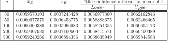
Table 4: Mean, standard deviation and confidence interval for error mean in Example 2 with m=16.
n xE sE %95 confidence interval for mean of E
Lower U pper
30 0.0059570103 0.0007245428 0.0056977360 0.0062162846 50 0.0060677570 0.0006453775 0.0058888675 0.0062466465 100 0.0060400389 0.0005996983 0.0058254355 0.0060605173 200 0.0059407980 0.0007160603 0.0058415571 0.0060400389 500 0.0059240266 0.0006894356 0.0058635949 0.0059844583
t∈[0,0.5), (46) with the exact solution
u(t) = 1 3e
−1
2t+12tln(t+1)+12ln(t+1)+
t 0
√
ln(s+1)dB(s),
for0≤t <0.5.
The numerical results are shown in Table 1 and Table 2. In tables, n is the number of iterations, xE is error mean, andsE is standard deviation of error.
Example 2. [15]Consider the following linear stochastic Volterra integral equation,
u(t) = 1 12+
t
0 cos(s)u(s)ds+
t
0 sin(s)u(s)dB(s)
t∈[0,0.5), (47) with the exact solution
u(t) = 1 12e
−t
4+sin(t)+sin8(2t+
t
0sin(s)dB(s),
for0≤t <0.5.
The numerical results are shown in Table 3 and Table 4.
8
Conclusion
As some SVIEs can not be solved analytically, in this article we present a new technique for solving SVIEs numerically. Here, triangular functions and their opera-tional matrix of integration are considered. The benefits
of this method are lower cost of setting up the system of equations without any integration, moreover, the compu-tational cost of operations is low. Also, convergence of this method is faster than BPFs [15] and order of con-vergence is O(h2). These advantages make the method easier to apply. Efficiency of this method and good rea-sonable degree of accuracy is confirmed by two numerical examples.
References
[1] J.A.D. Appley, S. Devin, and D.W. Reynolds, “Al-most sure convergence of solutions of linear stochas-tic Volterra equations to nonequilibrium limits,” J. Integral Equations Appl.19 (4) 2007, pp. 405-437. [2] E. Babolian, K. Maleknejad, M. Roodaki, and H.
Al-masieh, “Two-dimensional triangular functions and its applications to nonlinear 2D Volterra-Fredholm integral equations,”Comput. Math. Appl.60 2010 , pp.1711-1722.
[3] E. Babolian, H.R. Marzban, and M. Salmani, 2008. “Using triangular orthogonal functions for solving Fredholm integral equations of the second kind.” Appl. Math. Comput.201 2008, pp. 452-456. [4] E. Babolian, Z. Masouri, and S.
Hatamzadeh-Varmazyarb, “Numerical solution of nonlinear VolterraFredholm integro-differential equations via direct method using triangular functions,”Comput. Math. Appl.58 2009 , pp. 239-247.
[5] E. Babolian, Z. Masouri, and S. Hatamzadeh-Varmazya, “A Direct Method for Numerically Solving Integral Equations System Using Orthog-onal Triangular Functions,” Available online at
IAENG International Journal of Applied Mathematics, 43:1, IJAM_43_1_01
http://ijim.srbiau.ac.ir,Int. J. Industrial Mathemat-ics,1 (2) 2009, pp. 135-145.
[6] E. Babolian, R. Mokhtari, and M. Salmani, “Using direct method for solving variational problems via triangular orthogonal functions,”Appl. Math. Com-put.191 2007, pp. 206-217.
[7] M.A. Berger, and V.J. Mizel, “Volterra equations with Ito integrals I,” J. Integral Equations 2 (3) 1980, pp. 187-245.
[8] A. Deb, A. Dasgupta, and G. Sarkar, “A new set of orthogonal functions and its application to the analysis of dynamic systems.”J. Franklin Inst.343, 2006, pp. 1-26.
[9] Z. Han, S. Li, and Q. Cao, “Triangular Orthog-onal Functions for Nonlinear Constrained Optimal Control Problems”,Research Journal of Applied Sci-ences, Engineering and Technology,4 (12), 2012, pp. 1822-1827.
[10] F. C. Klebaner, Intoduction To Stochastic Calculus With Applications,I Monash University, Australia, Second edition 2005.
[11] P.E. Kloeden, and E. Platen, Numerical Solution of Stochastic Differential Equations,Applications of Mathematics, Springer-Verlag, Berlin, 1999. [12] K. Maleknejad, H. Almasieh, and M. Roodaki,
“Tri-angular functions (TF) method for the solution of Volterra-Fredholm integral equations,” Communica-tions in Nonlinear Science and Numerical Simula-tion, 15 (11) 2009, pp. 3293-3298.
[13] K. Maleknejad, and Z. JafariBehbahani, “Appli-cations of two-dimensional triangular functions for solving nonlinear class of mixed Volterra-Fredholm integral equations,” Mathematical and Computer Modelling.
[14] K. Maleknejad, M. Khodabin, and M. Rostami, “A numerical method for solving m-dimensional stochastic ItVolterra integral equations by stochas-tic operational matrix,” Computers and Mathemat-ics with Applications,2012, pp. 133-143.
[15] K. Maleknejad, M. Khodabin, and M. Rostami, “Numerical Solution of Stochastic Volterra Integral Equations By Stochastic Operational Matrix Based on Block Pulse Functions”,Mathematical and Com-puter Modelling 2012, pp. 791-800.
[16] B. Oksendal, Stochastic Differential Equations, An Introduction with Applications, Fifth Edition, Springer-Verlag, New York, 1998.
[17] E. Pardoux, P. Protter, “Stochastic Volterra equa-tions with anticipating coefficients,”Ann. Probab.18 1990, pp. 1635-1655.
[18] Y. Shiota, “A linear stochastic integral equa-tion containing the extended Ito integral,” Math. Rep.Toyama Univ, 9 1986, pp. 43-65.
[19] J. Zheng, S. Gan, Xi.Feng, and Dejun Xie, “Optimal Mortgage Refinancing Based on Monte Carlo Sim-ulation,” IAENG International Journal of Applied Mathematics,42 (2), 2012, pp. 111-121.