A dynamic life cycle analysis for a Defined Contribution pension plan

(1)

U

NIVERSITY OF

T

WENTE

F

INANCIAL

E

NGINEERING AND

M

ANAGEMENT

M

ASTER THESIS

A dynamic life cycle analysis for a

Defined Contribution pension plan

Author:

E.J. Knol

External supervisors:

K. Lee

M. Maradona

UT supervisors:

B. Roorda

R.A.M.G. Joosten

(2)

(3)

Management summary

Pension is an important part of our social security. Pension funds are under enor-mous pressure and pension cuts seem unavoidable without political interference. PME and PMT have already announced that cuts in 2020 are very likely. The cur-rent Defined Benefit pension system is under review and the market shifts towards a Defined Contribution pension plan, with more emphasis on individualisation. Such pension plans are still relatively new and therefore more research is needed in this area. This shift increases the importance of life cycle investing. A life cycle in-vestment strategy attempts to determine the most appropriate asset mix for Defined Contribution pension plan participants to balance their risk and return profiles based on the number of years the participants have until retirement. We have found no substantiation for the fact that the current life cycle performs well under the current economic conditions and leads to an optimal pension benefit. We have contributed to the literature because we have compared existing life cycles with optimised linear and dynamic life cycles, while in the current literature one of them is usually taken. The design of a dynamic life cycle has not yet been evaluated in the Dutch pension context. This explains the relevance of this research and the answer on the following main research question:

How should the life cycle be designed for a Defined Contribution pension plan?

In order to answer this question we have developed a method to analyse Defined Contribution life cycles. We started with capital calculations to gain insight into the capital development during the working period of a participant. This is used to cal-culate the ratio between the accumulated capital and the discounted value of the expected pension benefits, called the coverage ratio. Note that this coverage ratio is not the same as the definition used in a Defined Benefit pension system. The cov-erage ratio serves as an input for the constant relative risk aversion utility function. The utility is used to compute the certainty equivalents to compare the different life cycle designs. In addition to the assessment framework, we have built a simulation model to model the interest rate and equity returns. We have used the dynamic Nelson-Siegel model in combination with a vector autoregression model to simulate

(4)

IV MANAGEMENT SUMMARY

these interest rates and equity returns. The addition of a Markov regime switching component to the simulation model is of added value because it provided insight in how dynamic life cycles can be designed depending on the state of the economy.

We have showed with the analysis of the traditional, reverse, and constant life cycles that the currently most used life cycle, the traditional life cycle, should not be seen as a guarantee for the optimal pension result. Which life cycle is preferred depends on the risk aversion of a participant. The reverse, constant, and traditional life cycles are preferred for the low, medium, and high risk aversion perception respectively. This finding suggests that determining the risk aversion of a participant is of great importance.

In the second part of the life cycle analysis we have performed the optimisation with the goal to maximise the average utility by changing the life cycle. First, this is done for linear life cycles. We have found that the optimised linear life cycles result in higher utility values than the three existing life cycles. The shapes of these life cycles are completely different than the existing life cycles. In case a participant has a low risk aversion most capital is allocated to the return portfolio with a slight decrease over time. For the medium risk aversion profile the life cycle starts with an allocation of around zero percent to the return portfolio and increases to almost forty percent to the return portfolio at the end. In case a participant has a high risk aversion then the return portfolio allocation starts at zero percent and increases to almost twenty percent. These results, together with the sensitivity analysis, have showed that the linear life cycle design is highly dependent on the risk aversion coefficient, especially for the low risk aversion profile. This research goes beyond a linear life cycle which is only a function of age. The dynamic life cycle does not necessarily have to be a linear function and is state dependent in order to incorporate the market conditions in deciding the return portfolio allocation. It appeared that adding these two elements to a life cycle result in higher utilities and more certainty, in terms of coverage ratio, compared to a linear life cycle.

(5)

List of acronyms

AOW State guaranteed pension

CE Certainty Equivalence

CR Coverage Ratio

CRRA Constant Relative Risk Aversion

CVAR Conditional Value At Risk

DB Defined Benefit

DC Defined Contribution

DNB The Dutch Bank

DNS Dynamic Nelson-Siegel model

ECB European Central Bank

EPB Expected Pension Benefit

EURIBOR Euro Interbank Offered Rate

FV Future Value

GDP Gross Domestic Product

HICP Harmonised Index of Consumer Prices

LC Life Cycle

MSCI Morgan Stanley Capital International

NS Nelson-Siegel

OLS Ordinary Least Squares

PME Pension fund MetalElektro

(10)

X LIST OF ACRONYMS

PMT Pension fund Metaal & Techniek

PV Present Value

RQ Research Question

SBK Strategic Investment Framework

(11)

List of Figures

1.1 Problem cluster. . . 6

1.2 Research design. . . 10

2.1 Capital calculations. . . 15

2.2 Accruing the premiums. . . 18

2.3 Discounting the benefits. . . 18

3.1 Historical EURIBOR interest rate percentages (Home Finance, 2019). 24 3.2 Historical equity returns. . . 25

3.3 Flowchart simulation model. . . 26

3.4 Factor loadings DNS modelγ = 0.0609(Diebold & Li, 2005). . . 27

3.5 Graphs regime switches. . . 33

4.1 Traditional, constant and reverse life cycle. . . 41

5.1 Optimised linear life cycles. . . 49

5.2 Dynamic life cycle low risk aversion. . . 51

5.3 Dynamic life cycle medium risk aversion. . . 51

5.4 Dynamic life cycle high risk aversion. . . 52

5.5 Optimised linear life cycles using different risk aversion coefficients. . 54

(12)

(13)

List of Tables

1.1 Overview Dutch pension system. . . 3

3.1 Coefficient matrix State 1. . . 32

3.2 Coefficient matrix State 2. . . 32

3.3 Transition probability matrix. . . 33

3.4 Starting values simulation. . . 34

4.1 Coverage ratios given deterministic interest rates and equity returns. . 42

4.2 Certainty equivalents given stochastic interest rates and equity returns. 43 4.3 Statistics of the existing life cycles. . . 44

5.1 Certainty equivalents of the optimised linear life cycles. . . 50

5.2 Certainty equivalents of the dynamic life cycles. . . 52

5.3 Statistics of the dynamic life cycles with low risk aversion. . . 53

5.4 Statistics of the dynamic life cycles with medium risk aversion. . . 53

5.5 Statistics of the dynamic life cycles with high risk aversion. . . 53

5.6 Life cycles with different excess return calibrations. . . 55

D.1 Covariance matrix State 1. . . 70

D.2 Covariance matrix State 2. . . 70

(14)

(15)

Chapter 1

Introduction

In essence, a pension contract is a straightforward product. A premium is paid during working years in exchange for a pension benefit after retirement. A pension fund invests all the collected premiums and strives to get a good investment return while taking the risk into account. However, this long-term process is accompanied by uncertainties and difficulties to design a solid and future-proof pension system. The Dutch pension system is seen as one of the best in the world but is nevertheless currently a subject of the political debate. The current collective pension system is under review and the market shifts more towards an individualised pension plan. Because such pension plans are still relatively new, there is the need to do research into an individualised pension plan.

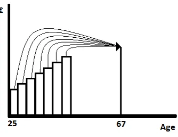
Currently, the market shifts from a current collective pension (Defined Benefit) plan towards a more individual pension (Defined Contribution) plan. In a Defined Contri-bution (DC) pension plan the investment strategy is commonly referred to as a life cycle. A life cycle investment strategy attempts to determine the most appropriate asset mix for DC plan participants to balance their risk and return profiles based on the number of years the participants have until retirement. In the traditional life cycle, which is the most used life cycle in a DC pension plan, more capital is allocated to the return portfolio in the beginning of the accumulation phase. This return portfolio is then linearly substituted for a more matching-like portfolio as the retirement date approaches. But is this actually the optimal life cycle? Does this life cycle result in the optimal pension, given the current market conditions and low interest rate en-vironment? The increasing importance of DC plans and their life cycles justify this research.

This opening chapter focusses on the framework surrounding this research. First of all, in Section 1.1 we give a short introduction about the organisation. Subsequently,

(16)

2 CHAPTER 1. INTRODUCTION

some background information is provided about the Dutch pension landscape. In Section 1.3 we cover the problem analysis which leads to a problem statement. Section 1.4 and 1.5 are devoted to the research questions and research design respectively. Thereafter, in Section 1.6 we briefly address the scope of this research. Finally, we give a rough thesis outline in Section 1.7.

1.1 Company profile

MN is the fiduciary manager for the Dutch manufacturing industry and the maritime sector. In terms of asset under management they are the third largest in the Nether-lands and the largest in the sector. MN managese135 billion in assets for more than 2 million people and are committed to their future income (MN, n.d.). The client list of MN includes Pension fund Metaal & Techniek (PMT), Pension fund MetalElektro (PME) and Koopvaardij. MN is a large company with close to a thousand employees and several business units.

This research fits to the business unit portfolio management under the Investment Strategy (Dutch: Strategisch Beleggingsbeleid) of the fiduciary advice department. The core task of fiduciary advice is to empower the members of the pension fund board making the right decisions in the field of portfolio management through good research which is then translated into policy advice and product development. This department is also responsible for writing investment strategies and mandates for implementation.

A pension fund board is responsible for the investment policy and makes use of supporting parties for advice and implementation. Central to the MN approach is a modern and effective investment framework. In 2015 this investment framework has been formalised into the ”Strategisch Beleggingskader” (SBK). In the framework the objective of the pension fund has been stated and how it wants to achieve the goal. A unique aspect of this approach is that MN prepares the SBK for all clients in a document in close consultation with the board. It forms the basis for the role as a fiduciary manager.

(17)

1.2. DUTCH PENSION LANDSCAPE 3

1.2 Dutch pension landscape

After seven years the Dutch pension system is again the number one pension sys-tem in the world according to the Global Pension Index 2018 (Mercer, 2018). Since 2009 Mercer compares the quality of pension systems over thirty countries world-wide and is based on three basic elements: adequacy, future-proofing, and integrity. This ranking indicates that the Dutch pension system is doing really well.

The three pillars

The Dutch pension system consists of three pillars. The first pillar concerns the state-guaranteed pension (AOW) which was introduced in 1957. It is the basic in-come and everyone who lives or works in the Netherlands will receive AOW as soon as the legal retirement age has been reached. The first pillar is financed through a pay-as-you-go system. This means that the working population pays the cost of the AOW of the current pensioners. The second pillar is a collective pension system organised around a specific industry/company. This is funded by the premiums that people have invested in the past, plus the return on it. If the employer has such a supplementary pension scheme, retired employees will receive an additional bene-fit on top of the AOW. The third pillar concerns the individual pension products. In particular, employees in sectors without a pension scheme and self-employed make use of this pillar. Our research focusses on the second pillar of the Dutch pension system.

First pillar State pension Pay-as-you-go Second pillar Occupational pension Funded

Third pillar Individual pension Funded

Table 1.1: Overview Dutch pension system.

Defined Benefit and Defined Contribution

(18)

(indexa-4 CHAPTER 1. INTRODUCTION

tion policy), with a negative indexation as the ultimate variant. The viability of a DB pension system is questionable and is one of the reasons why the current pension system is under discussion.

A Defined Contribution (DC) pension plan is a bit more straightforward. In a DC, the employee and employer contributions are invested on behalf of the employee (Hull, 2015). However, in a DC it is not known in advance what the exact pension benefit will be after retirement. Of course, this depends on the amount contributed but also on the growth of the capital throughout the years. Once the employee retires, the capital can be converted to a lifetime annuity. Because the pension benefit highly depends on the returns it increases the importance of the investments. This is where the life cycle comes into play. This is an investment policy which is often based on a function of the age of the (active) participant.

The majority of the sector in the Netherlands uses the DB pension system. However, numerous alternatives are the subject of discussion in politics and the pension in-dustry. One of the alternatives is a personal pension account with a collective buffer. This alternative can be seen as a hybrid between a DB and DC.

An important difference between DB and DC is the fact that the latter is a more individual kind of pension system. This can be seen as an individual employee account where the pension benefit is calculated based only on the funds on that account. This is in contrast with a DB pension system where there are no such individual accounts. The contributions are pooled and invested and the pension benefits are paid from the pooled capital. Another big difference is the way the risks are borne. With a DC plan the risk is fully carried by the employee because the pension benefit directly correlates with the total amount of capital of the individual fund. However, an advantage of a DC system is the flexibility. It can be adjusted based on personal characteristics which is not possible with a DB pension system.

1.3 Problem analysis

(19)

1.3. PROBLEM ANALYSIS 5

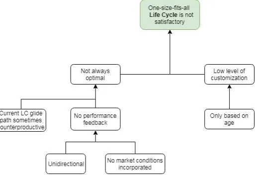
Because of the increasing social and political pressure, MN is interested in the ques-tion whether a hybrid pension system, which incorporates good elements of both the DC and DB systems, can meet the objectives. Right now the scope of this question is still quite broad and therefore it is necessary to narrow it down. Based on the preferences of MN, our research zooms in on the life cycle of the DC system. Ques-tioning the current life cycle is enhanced by literature pointing out that more research needs to be done to improve the current life cycle. There are already some stud-ies that evaluated life cycle designs of a DC pension plan, but they are somewhat outdated and therefore not representative for the currently low interest rate environ-ment, for example the study of Blake et al. (2001). However, these papers did not investigate a dynamic life cycle with the same definition as in this study. Next to that, Basu et al. (2011) stated that the LC can be counterproductive when moving away from stocks to low-return assets just when the size of the contributions are growing larger. They tested a dynamic life cycle where it is only allowed to switch between stocks and bonds during the last ten or twenty years. So, our study differs from their research in the definition of the dynamic life cycle. Another article stated that there is room for added value for the one-size-fits-all LC to incorporate classes of investors characteristics such as risk attitude and income (EDHEC-Risk Institute, 2011). In addition to that, the current LC does not incorporate investment results that are very dependent on market behaviour (Arnott et al., 2013). This means that there is no feedback or performance check built in the investment strategy which can have influ-ence on the remaining part of the LC. Poterba et al. (2006) found that the distribution of retirement wealth associated with typical life cycle investment strategies is similar to that from an age-invariant asset allocation strategy. They stated that it might be useful to compare the optimal life cycles with the existing ones. This literature study shows that there is indeed room for improvement and could be seen as an invitation to join the research about the life cycle.

(20)

[image:20.595.171.430.69.245.2]

Figure 1.1: Problem cluster.

1.4 Research questions

At the time of writing this report, the Dutch pension system is still under review. As the third biggest fiduciary manager in the Netherlands it is important for MN to build a sustainable pension plan, especially given the changing pension landscape.

One of the aspects being discussed in the review is the shift from a Defined Benefit pension plan towards a Defined Contribution pension plan. This trend stems from the more flexible labour market, longevity and ageing population. In addition to that, low interest rate environments have put more pressure to the coverage ratio (CR) of the majority of Defined Benefit schemes in the Netherlands. With the sustainability of the current DB plan being questioned and the trust in the system diminishing, there is an increasing pressure to look into another system such as Defined Contribution plans.

The shift from DB plans to DC plans presents a new challenge for fiduciary man-agers such as MN to advise the pension board how to best manage the retirement assets. In addition to the policy regarding employees contribution, the investment strategy/asset allocation decisions play an important role in determining the pension outcome. The increasing importance of DC plans and its life cycle justifies the need for this research.

(21)

1.4. RESEARCH QUESTIONS 7

bond-like assets (matching portfolio) according to a certain fixed glide path. Cur-rently, this glide path is a function of the participant’s age. To achieve the research objective, we have formulated several research questions. These serve as the ba-sis, guideline and structure for this thesis. We define the main research question as follows:

How should the life cycle be designed for a Defined Contribution pension plan?

An important aspect here is the question when the life cycle is optimal. On one hand, it is clear that a higher pension benefit is better than a lower pension benefit. On the other hand, more certainty in terms of the pension payment is better than less certainty. The problem is that these two outcomes are often substitutes: a higher benefit is usually accompanied by more uncertainty. Therefore, it is necessary to look at the trade-off between risk and return to see which life cycle offers the best result. The main research question is broken down into two research questions. These form collectively an answer to the main research question.

Research question 1

Which life cycle design offers the best return trade-off given a certain risk-aversion level of the participant and stochastic interest rates and equity returns?

(22)

Research question 2

What is the impact of adjusting the return versus matching portfolio based on the target pension benefit throughout the working life of the participant?

In this next step of the analysis we propose a new method. Instead of looking at the age of the participant (or the time to retirement) as an anchor point for determining the asset mix, the proposed life cycle defines the asset mix based on the extent to which the target pension benefit is achieved. At each point in time (for example each year) the value of the pension contribution is evaluated against the value of accruals at retirement. As the ratio of the contribution to accruals is higher (i.e. the pension contribution matches the pension payout) a bigger portion of pension benefit is secured by allocating more to the matching portfolio. This is done irrespective of the age of the participant at that point. Based on this idea, we expect that a dynamic life cycle, in which the allocation between return and matching portfolio is managed against the target pension benefit throughout the accumulation phase, generates a better pension result than the traditional life cycle in which the allocation is defined only based on the age of the participant.

Both research questions are related to the design of a life cycle for a DC plan and contribute in their own way to answering the main research question. In the next section we elaborate on the research design.

1.5 Research design

The research design serves as a roadmap for the entire process to achieve the re-search objective. Here, we break down the rere-search questions into smaller steps. We conduct the analysis through an iterative process, each time with small adjust-ments. In this way the impact of the incremental changes in the analysis can be isolated. In this research we explain and clearly state all assumptions for replication purpose. The main methods and data sources we use are literature studies, the MN pension database, extern data portals such as Bloomberg and the MN employ-ees. Knowledge about the pension industry is gathered through discussions and conversations with MN specialists. In the following paragraphs we elaborate on the different steps that we take to answer the research questions.

(23)

1.5. RESEARCH DESIGN 9

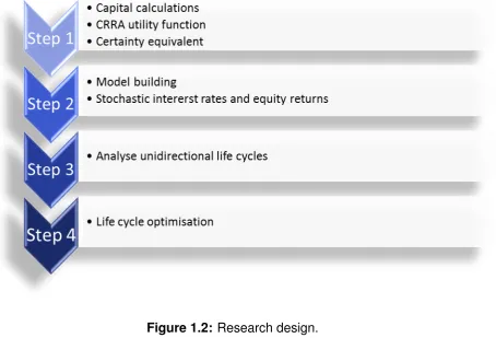
are made during the participant’s working years in exchange for a pension benefit after retirement. Therefore, it is fundamental to do the capital calculations to see how the total accumulated capital will change over time. Next to that, we use the Constant Relative Risk Aversion (CRRA) utility function which is one of the most commonly used utility functions in the pension industry (Yue, 2014) and is often used as an evaluation measure in the literate on dynamic asset allocation. The capital calculations, the CRRA utility function, and the certainty equivalents form the basis for the analysis of life cycle design. In order to conduct this analysis, data from the MN database is used as input. This includes the mortality table, career path percentages, and pension contribution table.

The goal of the second step is to be able to test the life cycle designs under different economic circumstances. We need to generate stochastic interest rates and equity returns to create a more realistic view of the performance of the life cycles. We do some literature study to gain knowledge about different models such as Vasicek, Nelson-Siegel (NS), Heath-Jarrow-Morton framework (HJM), Geometric Brownian Motion (GBM) and Markov regime. Given the scope of this research, we keep the scenario generation relatively simple. This also reduces the dependency on large amount of data. We gather the input data for scenario generation, for example data about swap rates and indices, using Bloomberg.

We use the results of the previous two steps in the third step to analyse three existing unidirectional life cycles. Once we have modelled the capital calculations, utility function, interest rates and equity returns, we test different life cycles to answer Research Question 1. These are referred as the constant, traditional and reverse life cycles, which we discuss in more detail in Chapter 4.

(24)

[image:24.595.84.539.138.447.2]

To summarise, we execute several steps to be able to answer the main research question. These steps together serve as a roadmap for this research. This can be represented in the following flowchart:

Figure 1.2: Research design.

1.6 Scope

(25)

1.7. REPORT OUTLINE 11

1.7 Report outline

(26)

(27)

Chapter 2

Assessment framework

As described in the first chapter our research consists of two research questions with the main objective to see whether a dynamic life cycle outperforms the current unidirectional life cycle. In order to answer the research questions we discuss the mechanism to capture risk-return trade-off first. The goal of this chapter is to come up with a risk-return measure to evaluate each of the life cycle design and to quantify the effect of changing the asset allocation mix. First, it is necessary to understand how the pension payout is calculated and what the pension contributions should be that the participant has to pay to achieve this pension payout objective throughout the accumulation phase. This is referred to as the capital calculations. In this calcu-lation the target pension payout at retirement date is set. We calculate the present value (PV) of the life-long benefit entitlements that are accrued by discounting the annual payout with the interest rates. The annual pension contribution (premium) is then calculated in such a way that at the target retirement date the future value (FV) of these premiums matches the present value of the annual pension payout. The same interest rate structure that is used to discount the pension payouts is used to calculate the future value of the contributions. The next step is related to the utility function. The risk aversion coefficient has to be determined in order to assess the life cycle using the utility function. Finally, the utility serves as an input in the cer-tainty equivalent (CE) calculation. We discuss all steps in more detail in the following sections.

2.1 Capital calculations

The participants pay pension contribution (premium) during their working years in exchange for a pension benefit after retirement. Currently, the retirement age is part

(28)

14 CHAPTER 2. ASSESSMENT FRAMEWORK

of the political discussion, so there is some uncertainty about what the retirement age will be in the future. For the purpose of this research we have assumed that the pension age is fixed. We have used the following inputs/assumptions in the capital calculations:

• The starting age for the wealth accumulation period is at the beginning of 25.

• The retirement age is at the beginning of 67.

• The last evaluated age is 103.

• The starting annual salary is e27,000.

• The franchise is e15,304.

• The payouts are at the beginning of a year (primo).

• The inflation correction is 0.5% per year.

• The career path is given as input.

• The mortality table is given as input.

• The pension accrual is 1.875% per year.

• The spot interest rate as of 29-3-2019 is used.

• Simulated interest rate and equity returns are used.

• The expected inflation term structure as of end March 2019 is used.

• No life events, like divorces or promotions, are incorporated.

• Partner pension is not taken into account.

(29)

[image:29.595.82.523.62.567.2]

2.1. CAPITAL CALCULATIONS 15

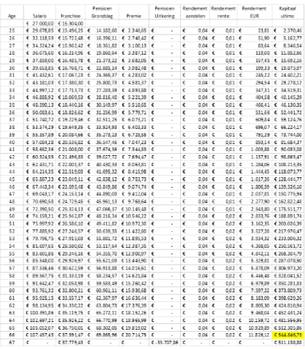
Figure 2.1: Capital calculations.

The first column is the age of the participant. We have calculated the capital on an annual basis starting with the year when the participant is 25 years old until he/she reaches the age of 103. We have chosen this lifetime range to accommodate the mortality table input; at the age of 103 the life expectancy is close to zero. The pension benefit is paid out at the beginning of the year. The retirement age kicks in when the participant reaches 67 (beginning of the year).

(30)

assump-16 CHAPTER 2. ASSESSMENT FRAMEWORK

tions that the starting salary ise27,000. At any year that the participant is younger than the retirement age (67) he/she earns a salary. The amount of salary changes over time depending on the inflation and the career path. We have assumed that the salary grows with the inflation. The career path shows the percentages with which the salary grows compared to the previous year as a result of a participant’s career.

The next column is the franchise computation. This is the part of the salary on which no pension is accrued and therefore no pension contribution (premium) is paid. It also depends on the starting value and is also effected by the inflation.

Next, the pension base (Dutch: pensioengrondslag) is calculated by deducting the franchise from the salary. The pension base is the part of the salary on which pension is accrued and therefore pension contribution is paid.

The next step is to calculate the pension contribution (premium) by multiplying the pension base with the accrual percentage. As you can see in Figure 2.1, premium is only paid when the participant is 66 years old or younger. In addition to the returns on investment, the inflow of premiums is an important source of capital. The premium policy is one of the management tools that a pension board can use if necessary. In our research, however, we have not used the premium as a steering tool. We have used a fixed contribution table, which can be found in Appendix B. The contribution percentages are based on the accrual percentage of 1.875% per year and the spot interest rate of March 31, 2019. In other words, this pension contribution must be paid to build up 1.875% pension per year, assuming all capital is allocated to the matching portfolio. We have found that this results in a pension annuity of e33,707.68 and is used as the pension ambition in our research. This stylised framework offers a clearer insight into the influence of the life cycle designs on the pension result.

In the sixth column the pension benefit is calculated. Note that the participant only receives the benefit when he/she is 67 years or older. The pension benefit depends on the total accumulated capital so far and on the annuity factor (Dutch: koopsom). In this research an annuity factor is an one-time payment to buy a pension entitle-ment (Pensioen.com, n.d.). The annuity factor represents the amount of money that is now needed to be able to buy an annual of one euro pension entitlement which is distributed from retirement age until the participant dies.

(31)

how much in the return portfolio. In our research the matching portfolio consist of interest rate investments and the return portfolio consist of equities. Therefore, the total annual returns depend on the interest rates and the equity returns.

The last column is the final step to calculate the total accumulated capital. This is called the capital ultimo. It depends on the accumulated capital up to the previ-ous year, the contribution in the current year, the pension benefit paid out this year (if any), and the total annual return on investment. We have used this capital to calculate the pension benefit because it incorporates everything such as premium, pension benefit, and returns from the investment portfolio.

Annuity factor

As mentioned before, we have used the annuity factor to determine the pension ben-efit based on the accumulated capital. The necessary inputs to calculate the annuity factors are age, mortality rate, and spot interest rates. A mortality table shows, for every age, what the probability is that a person of that age will die. The mortality table can be found in Appendix C. By using the mortality table, it is possible to cal-culate the conditional probability of survival at a certain age. The probability that someone is still alive up until a certain age, multiplied by one minus the probability that a person will die at that age, gives the conditional probability of survival. In other words, it is the probability that a participant will survive given that the partic-ipant survived up to now. We have done this for every year, ranging from 25 until 103 years old, assuming that the participant is now 25 years old. These probabilities are needed to generate the expected pension payout table with two dimensions, the current age of the participant and the time horizon. Given a certain age the expected pension payout is calculated. This is done by multiplying thee1 pension entitlement per year (annuity) with the probability that the participant is still alive each year. So, for example given that a person is now 60 years old (t = 35) and the horizon is 7 years (h = 7), what is the expect pension payout? We have done this for every age and horizon to generate the expected pension payout table. The expected pension benefit (EPB), dependent on the current age and horizon, is given by:

EPBt,h =  



e1× Pt+h

Pt , t + h≥67

0, t + h<67

, (2.1)

whereP is the probability of survival at a current aget ∈ {25,26, ...,103}and horizon h∈ {0, Z+}.

(32)

formula to calculate the annuity factorAis given by:

At=EP Bt,0+

T

X

h=1

EP Bt,h

(1 +rh)

h , (2.2)

whererh is the spot interest rate with a horizonh.

Now that these annuity factors are calculated we can use them to compute the pension benefit given the accumulated capital so far. This step serves as an input for the capital calculations.

Discounting cash flows

[image:32.595.83.265.414.554.2]

As mentioned in the previous section, the payments of the pension contribution and the pension benefit take place at different moments in time. This means that we need to accrue the contribution payments and to discount the pension benefits to be able to fairly compare the available money and liabilities at the retirement age. This gives an indication about the solvency of the pension fund at the time the participant retires. Figure 2.2 and Figure 2.3 give a schematic overview how the different cash flows are accrued and discounted.

Figure 2.2: Accruing the premiums. Figure 2.3: Discounting the benefits.

The premiums are paid annually and therefore the number of years until retirement decreases annually. This means that the premium paid by a participant at the age of 25 is invested for a period of 42 years while the premium paid at the age of 26 is invested for a period of 41 years and so on.

[image:32.595.319.481.415.553.2]

(33)

derived from the term structure of the spot interest rate. We have used the equation below to calculate the forward rates using the spot interest rate.

Fa+h =

(1 +ra+h)a+h

(1 +rh)h

_a1

−1, (2.3)

where r is the spot interest rate, a is the time to maturity (in years), and h is the horizon (in years).

This forward rate can be interpreted as the spot interest rateh years into the future with a time to maturitya. Using this formula, we have filled a two dimensional forward rates matrix with the dimensionstime to maturity andhorizon. The time to maturity, as its name already suggest, is the number of years until the investment is settled. The horizon, on the other hand, can be seen as moving the settlement date further into the future. So, for example whenh = 43 anda = 1, it means that the investment is settled at the corresponding forward rate for a period of one year at the beginning of age 68. This is because the payments are made at the beginning of the year. As already mentioned before, the capital calculations start at the beginning of age 25.

Once the forward rates have been calculated, they are used to accrue the premiums and to discount the pension benefits as showed in Figure 2.2 and Figure 2.3. For every payment the time to maturity and horizon will be determined to see which forward rate is applicable.

After accruing the investment portfolio and discounting the benefits, it is possible to see what the total future value of the invested premiums and the present value of the pension benefits is at retirement age. This gives an indication about the coverage ratio. To recall, the coverage ratio is the relationship between the current available capital and the future pension obligations. Note that the term coverage ratio is used in our research loosely and does not correspond to the definition of coverage ratio used in the DB system. The coverage ratio says something about the relationship between the premiums and the expected pension benefit. We have used this ratio as a solvency measure and serves as an input in the utility function. In the following section we explain the relationship between the utility function and the coverage ratio in more detail. To compute the coverage ratio we have used the following equation:

xt= It Bt

, (2.4)

(34)

The investment portfolio in the formula above can be seen as the future value of the invested premiums (see the last column of Figure 2.1). The life cycle represents the percentage allocated to the return and matching portfolio and thus has an influence on the investment portfolio. In addition, we have incorporated the probability of sur-vival in the present value calculation of the benefits because there is a chance that the participant dies earlier. The pension benefits are first multiplied by the probability of survival before discounting. It is the probability of survival given that the partici-pant has reached the retirement age. This means that the pension benefit received at the beginning of 67 is multiplied by one because the probability of survival given that the participant reached the retirement age is one. The pension benefit at the beginning of 68 is multiplied by 0.9857 (mortality rate is 1.43% at the age of 67) because that is the probability the participant will receive the pension benefit. This is done up to the age of 103.

2.2 Measures

In economics, the utility function measures the welfare or satisfaction of a consumer as a function of consumption (Investopedia, 2018). In this case, the consumption is in terms of CR because it serves as a solvency indication of their pension. As we have already stated in the introduction chapter, we have used the Constant Relative Risk Aversion (CRRA) utility function, which is according to Yue (2014) one of the most commonly used utility functions in the pension industry. As the name already somewhat implies, risk aversion is the concept of human behaviour of disliking un-certainty. To give an example, if a player gets two options, a guaranteed payment of

e50 or a 50% chance one100 and 50% chance one0, a highly risk-averse player will choose the guaranteed payment while the expected payouts are both the same. A risk neutral player would be indifferent between the two options. Someone’s risk aversion is incorporated in terms of a risk aversion coefficient in the utility function. The CRRA utility function is defined as follows:

U(x) = x

1−γ

1−γ , (2.5)

wherex is the coverage ratio andγ is the risk aversion coefficient.

(35)

2.3. CONCLUSION 21

real risk aversion coefficient is for everyone and to compute the utility function on an individual basis. Instead, we have created three profiles with different risk aversion coefficients, based on the paper of EDHEC (2014). We have used the following risk aversion profiles:

• Low risk aversion (offensive),γ = 2.

• Medium risk aversion (neutral),γ = 5.

• High risk aversion (defensive),γ = 10.

The utility values for every risk profile can be compared in order to determine the life cycle preferences. Interpreting one single utility is difficult because what does an utility of minus one, for example, mean? To get more feeling about the results we have used the certainty equivalent measure. This transforms a distribution of uncer-tain outcomes into a single value with probability one that has the same utility. It can be interpreted as a guaranteed CR that someone would accept rather than taking a chance on a higher, but uncertain, CR in the future. After determining the expected utilities it is straightforward to determine the certainty equivalent. Ranking alterna-tives by certainty equivalents is the same as ranking them by their expected utilities. Rewriting Formula 2.5 results into the following certainty equivalent equation:

C= (E(U)×(1−γ))1−1γ , (2.6)

whereE(U)is the expected utility andγ ∈ {2,5,10}is the risk aversion coefficient.

2.3 Conclusion

(36)

a pension benefit ofe33,707.68. We have assumed that this is the lifetime annuity regardless of the fact that the asset allocation mix will change later in our research.

In addition, we have used the utility function to assess the trade-off between risk and return and to be able to compare the different life cycles fairly. We discuss the three existing unidirectional life cycles, which are tested later on in this research, in more detail in Section 4.1. They differ in terms of riskiness. Riskier life cycles might result in a higher pension benefit but at the same time have a greater chance on a terrible pension entitlement. In case a participant has already a good pension prospect then it might not be worth it to take extra risk to get an even better pension benefit. Besides that, not everyone is willing to take the same risk. Determining the risk aversion of every individual is not the goal of our research. Based on this rea-son, we have created three risk aversion profiles (defensive, neutral, and offensive) with their own risk aversion coefficient. The utility function is a useful measure for comparing the life cycles but the values do not say anything in itself. Therefore, we have transformed the utilities into certainty equivalents to be able to better interpret the results.

(37)

Chapter 3

Model building

We have built a simulation model to test the life cycles using stochastic interest rates and equity returns as input, which we discuss in this chapter. First, we give a short introduction about interest rates and equity returns. This emphasises the importance to use stochastic interest rates and equity returns. In Section 3.2 we explain the simulation model step by step, which consists of a dynamic Nelson-Siegel and a vector autoregression (VAR) model with a Markov regime switching component. The addition of a Markov regime switching component is not done a lot in the literature and therefore can be seen as an innovative element.

3.1 Interest rate and equity returns

The interest rate has a huge impact on the economy, and also on the pension indus-try. For the pension industry interest rates are used as input variable for calculating the values of the pension liabilities. Pensions are accrued over a long period and are usually paid for quite a long time. In determining the pension liabilities, pension funds must therefore use a long-term interest rate prescribed by the Dutch bank (DNB). Currently, the interest rates are historically low, around zero or even slightly negative. The interest rate drop is significant as can be seen in Figure 3.1. Be-cause of the low interest rate, pension funds are obliged to have more money in cash than, for example, a few years ago. This puts an enormous pressure on the pension industry and is also one of the reasons why the current pension industry is being discussed.

(38)

[image:38.595.177.416.68.251.2]

24 CHAPTER3. MODEL BUILDING

Figure 3.1:Historical EURIBOR interest rate percentages (Home Finance, 2019).

Because of the high importance of the interest rate a lot of research has been con-ducted to be able to model interest rate movements. These researches can es-sentially be classified into two frameworks. The first framework is to model the interest rate by modelling the evolution of the short rate. Under a short rate model, the stochastic state variable is taken to be the instantaneous spot rate (Wikipedia, 2019). From the short rate an entire yield curve is built up. If one chooses to fit the resulting interest rates on the current yield curve, the parameters of the model have to be calibrated to be consistent with the current observed prices of interest rate instruments. Well-known one-factor short rate models are for instance:

• Vasicek model (1977).

• Cox-Ingersoll-Ross model (1985).

• Ho-Lee model (1986).

• Hull-White model (1990).

(39)

3.1. INTEREST RATE AND EQUITY RETURNS 25

interest rates (Bank for International Settlements, 2005). In addition, the model is parsimonious due to its simple functional form (see the formula in the next section) and can be extended to a no-arbitrage model.

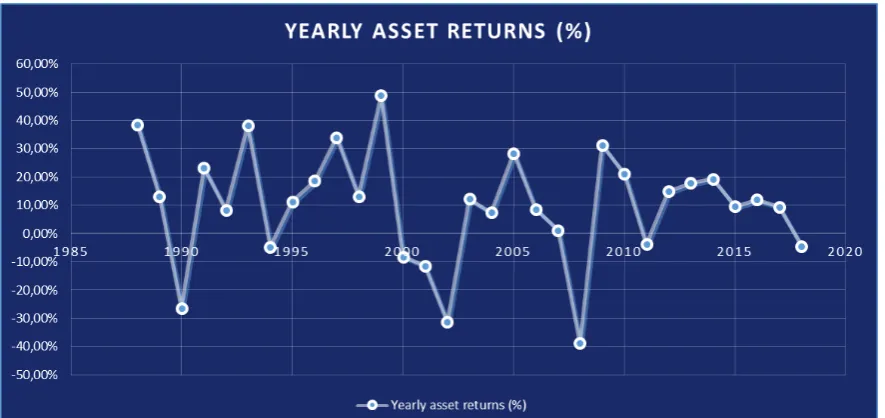
In addition to the interest rate, modelling the equity returns is also an important part of this research. The return on equity investments comes in the form of dividend payments or capital gains from the increase in equity prices. A lot of research has been done regarding stock price modelling. Prices can fluctuate considerably as expectation regarding earnings growth and risk premium changes. As investors are faced with high risks they also demand higher returns on equity investments.

[image:39.595.82.525.462.671.2]

We have used the MSCI All Country World Index as a proxy for worldwide equities. Figure 3.2 gives an overview of the annual total returns on equities. As can be seen from the figure below the returns fluctuate quite a lot, which illustrates the difficulty to predict the future returns. However, Sengupta (2004) wrote in his book: ”We talk about simulating stock prices only because future stock prices are uncertain (called stochastic), but we believe they follow, at least approximately, a set of rules that we can derive from historical data and our other knowledge of stock prices. This set of rules is called the model for stock prices”. We discuss our model used to ‘explain’ the interest rate and equity return paths in the next section.

(40)

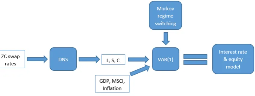
3.2 Simulation model

[image:40.595.88.511.285.444.2]

Simulations can be used to show the possible effects of alternative conditions but building a simulation model can be a complex thing to do. In the remaining of this section we explain our model step by step, see Figure 3.3 for an overview of the model. First, we explain the two underlying concepts, which are the dynamic Nelson-Siegel model and the Markov regime switching. Then we discuss some interim results, after which we explain the refinement and calibration of the model. We have used Matlab and Excel to build the simulation model. We do not discuss these codes in detail but they can be found in Appendix F.

Figure 3.3: Flowchart simulation model.

Dynamic Nelson-Siegel

(41)

3.2. SIMULATION MODEL 27

the following DNS formula to model the yield curve:

yt(τ) = β1,t+β2,t×

1−e−λ×τ λ×τ

+β3,t×

1−e−λ×τ λ×τ −e

−λ×τ

, (3.1)

whereyt(τ)is the yield with maturityτ at timet,λis the loading parameter, andβ1,β2 andβ3 are the level, slope and curvature factors respectively.

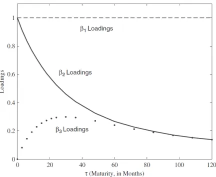
[image:41.595.190.406.500.677.2]

As can be seen in the formula above the loading parameter is not dependent on time, which simplifies the underlying assumptions of the model. The loading factor determines the exponential decay of the slope and curvature factor. The other vari-ables, the latent factorsβ1, β2, β3, are dependent on time. These betas are called level, slope, and curvature respectively and carry some level of economical inter-pretation (Koopman et al., 2012). The first component equally influences the short and long-term interest rate and can therefore be interpreted as the overall level. The second component converges to one if the maturity goes to zero and converges to zero if maturity goes to infinity. This indicates that this component influences mainly the short term interest rate. The third component is associated with medium term interest rates because it is a concave function which converges to zero if maturity goes to zero and also converges to zero if maturity goes to infinity. The loading parameter influences the moment when the third component reaches its maximum. Figure 3.4 gives an overview of the loading factors in relation to time to maturity. These three loading factors together can capture a lot of different kind of shapes observed in yield data.

Figure 3.4: Factor loadings DNS modelγ = 0.0609 (Diebold & Li, 2005).

(42)

monthly zero coupon swap rates from January 2000 through March 2019 with dif-ferent time of maturities using Bloomberg. These maturities are 1 up to 10-year, 12, 15, 20, 25, 30, 40, and 50-year. We have estimated the loading parameter using the optimisation toolbox of Matlab and the Ordinary Least Squares (OLS) method. OLS regression is a statistical method that estimates the relationship between a re-sponse variable and one or more explanatory variables. The method estimates the relationship by minimising the sum of the squares in the difference between the ob-served and predicted values of the response variable configured as a straight line, and is also referred as linear regression (Dickey et al., 2001). Initially, a loading pa-rameter is set in order to compute the error in the first iteration. In every iteration a loading parameter is chosen in order to compute the level, slope and curvature fac-tors. With these factors the swap rates are estimated which are then compared to the real data to calculate the error. For the next iteration the optimisation command in Matlab automatically chooses a new loading parameter and again computes the level, slope, and curvature factors to calculate the error. This process is repeated many times to find the optimal loading parameter which is the one with the minimum sum of squares. We have programmed this method in Matlab and the code can be found in Appendix F. The resulting loading parameter is 0.579, which we use in the remainder of our study. Finally, we have used this loading parameter to compute the time series of the level, slope and curvature factors. These time series are used to compute the parameters for the Markov regime switching.

Markov regime switching

(43)

an error term. The lagged variables are also referred to as the explanatory vari-ables. In this research we have used a VAR model with one lag (abbreviated as VAR(1)). Let’s assume that historical behaviour can be described adequately with the following regression:

Yt=β1 Xt−1 +εt, (3.2)

whereεt∼N(0, σ2)

Now suppose that an event takes place that changes the level of the response vari-able Yt dramatically and cannot be linearly explained by Equation 3.2. Then the

formula above does not fit the historical behaviour anymore. The regression formula changes to:

Yt=β2 Xt−1 +εt, (3.3)

whereεt∼N(0, σ2)

The formulas above can be rewritten to a Markov regime switching model. If there arek states then there are k values for the coefficient and volatility. If there is only one state then the formula is the same as a linear regression model. The Markov regime switching formula can be written as follows:

Yt=βSt Xt−1 +εSt , (3.4)

whereStis State1,2,...,k andεSt ∼N(0, σSt 2₎_.

(44)

mathematically represented as follows:

P (Xn=in|X0 =i0, X1 =i1, ..., Xn−1 =in−1) =P (Xn =in |Xn−1 =in−1). (3.5)

In other words, all that matters to determine the probability of the current state is the knowledge of the previous state. All the information that could influence the future evolution of the process is fully captured by the present state. This information is stored in the transition matrix Π. We have assumed that Π is independent of time t. Every row of the transition matrix is a probability vector and must be equal to one because it is absolutely certain that the future state is either state i or state j (assuming a two state system). The(i, j)thelement is given by the following formula:

πi,j =P(Xt+1 =j |Xt=i). (3.6)

For example, consider a two state system where at a certain time t the state is 1. Then there is a probability (π1,2) of moving from State 1 to State 2 between timet and t+1. Likewise, there is a probability (π1,1) of staying in state 1. Mostly, the transition probabilities are assumed to be constant over time, but it is also possible to use changing transition probabilities called a time varying transition probabilities model. In this research we have assumed that the transition probabilities are constant over time. The transition probability matrix can be represented as:

Π =

  

π1,1 · · · π1,k

..

. . .. ...

πk,1 · · · πk,k

 

. (3.7)

Now that we have explained the basics of Markov regime switching models, the task remains to incorporate the methodology in the simulation model. We have used Per-lin (2015) as a guidePer-line for the implementation of a Markov switching component. The author created a Matlab package for the estimation, simulation and forecast-ing of a general Markov regime switchforecast-ing model. The technical explanation of the method is provided by Perlin (2015).

(45)

on the absolute level, slope, and curvature factors does not say anything about the regimes. The delta values are composed and used as input for the Markov switching regime model and provide information about the regimes. Higher deltas indicate a higher volatility regime. The delta level, slope, and curvature values are not the only three response variables. The other three response variables are the Gross Domes-tic Product (GDP), inflation and equity returns. This means that the VAR(1) model has a total of six equations with level, slope, curvature, inflation, GDP, and equity returns as the response variables and the lagged values of the just mentioned vari-ables as the explanatory varivari-ables. We discuss the specification of the data in the next paragraph. The VAR(1) model can be represented by the following equation:

Y =DSt

T _Z ₊_W

St , (3.8)

where Y, Z, and W are column vectors with dimension 6x1 representing the six variables. The response variables are represented by Y, the lagged explanatory variables by Z, and the random variables by matrix W ∼ N(0,ΣSt), which is state dependent. St is modelled with a Markov regime switching process with the help

of the MS Regress package of Perlin (2015). The outputs of the Markov regime switching are discussed later in this report. D is the coefficient matrix of State S at timet (see Table 3.1 and Table 3.2 for the coefficient matrix of State 1 and State 2 respectively).

Both the coefficients and the error term are state dependent. This means that the coefficients and variance are switching according to the transition probabilities. We have built this VAR(1) model with the help of the MS Regress package of Perlin (2015) to compute the coefficient matrices, the covariance matrices, and the transi-tion probability matrix.

Data

(46)

real economic growth excluding inflation. To measure inflation we have gathered the Eurozone seasonally adjusted Harmonised Index of Consumer Prices (HICP) monthly percentages from the European Central Bank (ECB) database. This vari-able measures the change over time in the prices of consumer goods and services acquired, used or paid for by euro area household. We have chosen to use season-ally adjusted data to provide a more accurate depiction of price movements void of anomalies that can occur during specific seasons. At last, we have used monthly All Country World Index from the MSCI database as a proxy for worldwide equity returns. This index captures the equity markets from 23 developed and 26 emerging markets and is therefore a good proxy for global equity benchmark. All data in this research covers the period from December 2000 to March 2019.

Output Markov regime switching

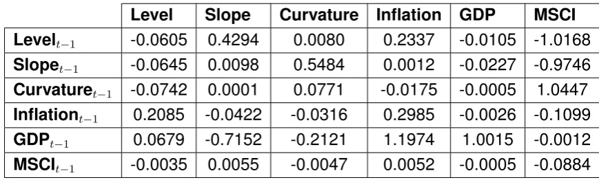
Up to now we have discussed the DNS model with the Markov switching regime component and the underlying data. In this step we have used the multivariate re-gression previously described and the MS Regress Matlab package of Perlin (2015) to compute the coefficients, transition probability, and covariance matrices. These are necessary in order to simulate the interest rates and equity returns. The two-state model entails two sets of coefficient matrices and covariance matrices. The coefficient matrices are represented in the following tables:

Level Slope Curvature Inflation GDP MSCI Levelt−1 0.0384 0.4527 0.0045 0.0660 0.0330 1.7158

Slopet−1 0.1836 0.2805 -0.4659 0.0152 0.0233 1.8861

Curvaturet−1 0.0537 0.00098 -0.0201 0.0077 0.0047 -0.2966

Inflationt−1 0.1037 -0.0533 -0.2557 0.3176 -0.0040 2.2860

GDPt−1 -0.1652 0.1641 0.1268 0.5358 0.9885 0.0106

[image:46.595.93.512.419.548.2]

MSCIt−1 0.0053 -0.0085 0.0143 0.0059 0.0006 0.10099

Table 3.1: Coefficient matrix State 1.

Level Slope Curvature Inflation GDP MSCI Levelt−1 -0.0605 0.4294 0.0080 0.2337 -0.0105 -1.0168

Slopet−1 -0.0645 0.0098 0.5484 0.0012 -0.0227 -0.9746

Curvaturet−1 -0.0742 0.0001 0.0771 -0.0175 -0.0005 1.0447

Inflationt−1 0.2085 -0.0422 -0.0316 0.2985 -0.0026 -0.1099

GDPt−1 0.0679 -0.7152 -0.2121 1.1974 1.0015 -0.0012

MSCIt−1 -0.0035 0.0055 -0.0047 0.0052 -0.0005 -0.0884

[image:46.595.78.513.580.711.2]

(47)

[image:47.595.125.478.309.496.2]

Based on the comparison of Table 3.1 with Table 3.2 we can conclude that there are differences between the coefficients of State 1 and State 2. The frequency of using the corresponding coefficient matrix depends on the probability of being in State 1 or State 2. The bottom graph in Figure 3.5 gives an overview of the probability of being in State 1 or State 2 over time. As can be seen, quite some switches occur between State 1 and State 2 in the beginning. Then the system stays in State 1 for a while, after which it switches again more often to State 2, followed by somewhat longer periods staying in State 1. The smoothing probabilities (bottom graph) can also be reconciled with the behaviour of the corresponding conditional standard deviation (middle graph). Where the higher volatilities of the financial crises of 2001 - 2003 and 2008 - 2009 are evident, throughout observation 0 - 25 and 85 - 100 approximately, the smoothing probabilities of both portfolios demonstrate that State 2 is probably the ‘bear’ regime.

Figure 3.5: Graphs regime switches.

The other Markov regime switching output is the transition probability matrix which gives the probabilities of going from one state to another state. This is given in the following transition probability matrix:

State 1 2

1 0.878 0.122 2 0.516 0.484

Table 3.3: Transition probability matrix.

(48)

because it is certain that the system will either stay in the same state or go to the other state. We have used this transition probability matrix, next to the coefficient and covariance matrices, to simulate the interest rates and equity returns.

Simulation

A simulation model can be used to determine the probabilities of outcomes, which cannot be determined or are difficult to determine analytically, because of the ran-domness of several input variables. Such a model can be used to simulate the in-terest rates and equity returns. The outcomes from the earlier analysis are needed to perform the simulation. These include the coefficient matrices, the covariance matrices, the two correlated random variables matrices and the transition probabil-ity matrix. The input data covers the period up to March 2019 and is therefore the last period that the data on the level, slope, curvature, inflation, GDP, and equity returns are known. We have used March 2019 data as a starting point of the sim-ulation, which is done on a monthly basis. As previously mentioned, we have used the delta values of the level, slope, and curvature factors to compute the Markov regime switching parameters. These delta values are also used to calculate the new delta values for the simulated periods. Then these new delta values together with the random variables are added to the absolute starting values. The random variables are correlated and therefore we have used the Cholesky decomposition, which can be found in Appendix D. The delta starting point and the absolute starting point are given in the table below. Note that delta and absolute values are the same for the inflation, GDP, and equity return data. This is because these are already month-over-month percentages.

[image:48.595.91.502.493.549.2]

March 2019 Level Slope Curvature Inflation GDP MSCI Delta -0.27% 0.36% -0.06% 0.110% 0.113% 2.75% Absolute 1.31% -1.00% -3.54% 0.110% 0.113% 2.75%

Table 3.4: Starting values simulation.

(49)

we have used the transition probability matrix to determine the next state. Let’s say the system is currently in State 1. To check whether the system will stay in State 1 or go to State 2, again a random number from the same distribution is drawn. If this random number is less than 0.878 then the system will stay in State 1 the next period. If the system is currently in State 2 and the random number is less than 0.516 then the system will go to State 1. If that is not the case the system will stay in state 2. So, in line with the Markov chain theory, the next state only depends on the current state and the transition probabilities.

So far it is clear in which state the system is. The next step is to compute the simulated values of level, slope, curvature, inflation, GDP, and equity returns. Based on the information whether the system is in State 1 or State 2, the corresponding coefficient matrix of State 1 or State 2 is used. Then by using Equation 3.8 we have calculated the level, slope, curvature, inflation, GDP, and equity return values for the next period.

As can be seen in the formula, the six response variables are dependent on the coefficient matrix, the values of the previous period, and the correlated random vari-ables matrix. Which coefficient matrix and correlated random varivari-ables matrix are used depend on the state of the system. We have used Equation 3.8 to calculate the new level, slope, curvature, inflation, GDP, and equity return values for every sim-ulated period. The number of simsim-ulated periods is 504 (42x12) because a 42-year interest rate and equity return forecast is needed for the capital calculations. In total five thousand simulations are done to assess the life cycles with different interest rate paths and equity returns.

The result of the previous step is a 504x6 matrix, which contain the values of the six factors, for every simulation. Now, we have simulated the equity returns and no further steps are required. On the other hand, an additional step is needed for the interest rate. Up to now, we have simulated the level, slope, and curvature values. However, these data are on a monthly basis whereas the capital calculations are on an annual basis. Therefore we have filtered the data first in such a way that only the yearly level, slope, and curvature values remain. Then we have used the DNS formula, see Equation 3.1, to construct the yield curves using the simulated level, slope, and curvature values and the previously determined loading parameter of 0.579. A figure showing the 30-year yield curves can be found in Appendix E.

Calibrating the model

(50)

we have calibrated the interest rate based on the forward rates. This means that the average of the yield curves should approximately the same as the forward rates based on the spot interest rate. As is described in Chapter 2 we have used the spot interest rate to calculate the forward rates using Equation 2.3. This will be referred as the forward rate matrix. In addition, the average yield curves of the five thousand simulations are calculated and is also a two dimensional matrix with the axeshorizon andmaturity. This matrix is then subtracted from the forward rate matrix. This result is added to the simulated yield curves every time the simulation is executed to make sure that the simulated yield curves are approximately consistent with the market observations.

The equity returns need to be calibrated as well and is done in the same way. This time it is somewhat less clear based on which value the equity returns should be calibrated. This is due to the fact that the current market observation does not necessarily mean that it is representative for the future. Therefore we have calibrated the equity returns based on the historical excess returns of 3.5%, which is based on a long-term return study (1814 - 2014) of the Deutsche Bank (2014). First, we have constructed a 5000x42 simulated equity return matrix with the dimensionssimulation run and horizon. A matrix with the same dimensions is also created but this time with the matching returns. How these matching returns are calculated is discussed in the next paragraph. Subsequently, we have substracted the equity return matrix from the matching return matrix, which results in an excess return matrix. Then for every horizon we have calculated the average excess return resulting in a 1x42 vector. These values should be approximately 3.5%. We have created a vector called delta equities by subtracting 3.5% from the 1x42 vector. This delta equities vector is then added to the simulated equity returns every time the simulation is executed. In this way the average simulated excess return is consistent with the historically observed excess returns.

Matching and equity returns

(51)

3.3. CONCLUSION 37

the return on the liabilities because we have calculated the expected pension bene-fits in such a way that these benebene-fits are achieved when all the capital is allocated to the matching portfolio. Therefore, the present values of the benefits can be seen as a theoretical price of the matching portfolio. Once we have calculated the ‘prices’, the price movements are computed as a result of the changing interest rates. This is done by calculating the present value changes. We have calculated the present value at the age of 25(t = 0)by using the spot interest rate, which means that it is the same in every run of the simulation. We have calculated the other present values by using the simulated yield curves. This means that at the age of 26 the expected cash flows are discounted with the simulated interest rate curve att = 1 and at the age of 27 the simulated interest rate curve at t = 2 is used and so on. In this way all present values are calculated, thus at the age of 25 till 67. The matching return formula is as follows:

Mt= Bt+1

Bt

−1, (3.9)

where M is the return on the matching portfolio and B is the present value of the benefits at timet.

We have done the matching and equity returns calculations for every simulation run. In this way the matching and equity returns are stochastic and can be used in the assessment of the life cycles.

3.3 Conclusion

(52)

(53)

Chapter 4

Life cycle analysis

Up to now we have modelled the capital calculations, utility function, interest rates and equity returns. This framework can now be used to test some existing unidi-rectional life cycles in order to answer Research Question 1. The research question that is central to this chapter is formulated as follows:

Which cycle design offers the best risk-return trade-off given a certain risk-aversion level of the participant and stochastic interest rates and equity returns?

To answer this question we introduce the different kind of life cycle designs first. This is done in Section 4.1. Once we have explained the life cycles we use the assessment framework and simulation model to test the life cycles. We have used Matlab and Excel to perform the analysis. The associated Matlab codes can be found in Appendix F. In Section 4.2 we interpret and discuss the empirical results.

4.1 Life cycle designs

Recall that a life cycle is the asset allocation mix during the accumulation phase that reflects the ratio between the matching and return portfolio. The accumulation phase is the period in which a participant accrues pension by paying a premium. The purpose of the matching portfolio is to replicate the change in value of the liabilities. Commonly used financial products for the matching portfolio are government bonds, corporate bonds and interest rate swaps. The purpose of the return portfolio is to maintain purchasing power by generating excess returns compared to the nominal obligations. One can think of equities, real estate investments, and high yield bonds

A dynamic life cycle analysis for a Defined Contribution pension plan

U

NIVERSITY OF

T

WENTE

F

E

M

M

A dynamic life cycle analysis for a

Defined Contribution pension plan

Author:

E.J. Knol

External supervisors:

K. Lee

M. Maradona

UT supervisors:

B. Roorda

R.A.M.G. Joosten

Management summary

Contents

List of acronyms

List of Figures

List of Tables

Chapter 1

Introduction

1.1

Company profile

1.2

Dutch pension landscape

1.3

Problem analysis

1.4

Research questions

1.5

Research design

1.6

Scope

1.7

Report outline

Chapter 2

Assessment framework

2.1

Capital calculations

2.2

Measures

2.3

Conclusion

Chapter 3

Model building

3.1

Interest rate and equity returns

3.2

Simulation model

3.3

Conclusion

Chapter 4

Life cycle analysis

4.1

Life cycle designs