warwick.ac.uk/lib-publications
Original citation:
Bradbury, Matthew S. and Jhumka, Arshad (2017) A near-optimal source location privacy
scheme for wireless sensor networks. In: 16th IEEE International Conference On Trust,
Security And Privacy In Computing And Communications (IEEE TrustCom-17), Sydney,
Australia, 1-4 Aug 2017. Published in: IEEE CPS Proceedings.
Permanent WRAP URL:
http://wrap.warwick.ac.uk/88960
Copyright and reuse:
The Warwick Research Archive Portal (WRAP) makes this work by researchers of the
University of Warwick available open access under the following conditions. Copyright ©
and all moral rights to the version of the paper presented here belong to the individual
author(s) and/or other copyright owners. To the extent reasonable and practicable the
material made available in WRAP has been checked for eligibility before being made
available.
Copies of full items can be used for personal research or study, educational, or not-for profit
purposes without prior permission or charge. Provided that the authors, title and full
bibliographic details are credited, a hyperlink and/or URL is given for the original metadata
page and the content is not changed in any way.
Publisher’s statement:
“© 2017 IEEE. Personal use of this material is permitted. Permission from IEEE must be
obtained for all other uses, in any current or future media, including reprinting
/republishing this material for advertising or promotional purposes, creating new collective
works, for resale or redistribution to servers or lists, or reuse of any copyrighted component
of this work in other works.”
A note on versions:
The version presented here may differ from the published version or, version of record, if
you wish to cite this item you are advised to consult the publisher’s version. Please see the
‘permanent WRAP URL’ above for details on accessing the published version and note that
access may require a subscription.
A Near-Optimal Source Location Privacy Scheme
for Wireless Sensor Networks
Matthew Bradbury and Arshad Jhumka
Department of Computer Science University of Warwick, Coventry,
United Kingdom, CV4 7AL
{M.Bradbury, H.A.Jhumka}@warwick.ac.uk
Abstract—As interest in using Wireless Sensor Networks (WSNs) for deployments in scenarios such as asset monitoring increases, the need to consider security and privacy issues also becomes greater. One such issue is that of Source Location Privacy (SLP) where the location of a source in the network needs to be kept secret from a malicious attacker. Many techniques have been proposed to provide SLP against an eavesdropping attacker. Most techniques work by first developing an algorithm followed by extensive performance validation. Differently, in this paper, we model the SLP problem as an Integer Linear Programming optimization problem. Using the IBM ILOG CPLEX optimiser, we obtain an optimal solution to provide SLP. However, that solution is centralised (i.e., requires network-wide knowledge) making the solution unsuitable for WSNs. Therefore, we develop a distributed version of the solution and evaluate the level of
privacy provided by it. The solution is hybrid in nature, in
that it uses both spatial and temporal redundancy to provide SLP. Results from extensive simulations using the TOSSIM WSN simulator indicate a 1% capture ratio is achievable as a trade-off for an increase in the delivery latency.
Index Terms—Source Location Privacy, Wireless Sensor Net-works, Optimal Routing, Integer Linear Programming.
I. INTRODUCTION
As wireless sensor networks (WSNs) are becoming increasingly viable for large scale deployments, applications such as asset monitoring and tracking can be implemented using this technology [1, 2]. In an asset monitoring application, the nodes in the network monitor their surrounding area to detect the presence of a valuable asset. When such an asset is detected a
message is transmitted from that sourcenode back to a base
station called the sink. As the range of the sensor nodes is
typically less than that between the source and sink, multiple hops need to be used for the message to reach the sink.
To protect the content of this data, messages can be
encrypted, however, the act of routing the message to the sink
revealscontextinformation about the event that encryption does
not and can not protect. One example of context information that needs to be protected is the location of the source, as revealing this information would allow an attacker to follow messages through the network to the source and capture it. The SLP problem was originally presented as the panda hunter game [3, 4]. In this situation pandas are being monitored by a WSN and information is being reported to conservationists working at a base station. Other situations such routing
messages between soldiers on a battlefield would benefit from applying SLP techniques.
Much work has been done on developing new routing strategies that provide SLP [5] since the seminal work. Most works first develop a technique before using simulations to demonstrate the performance of the technique and some works use techniques such as information theoretic analysis to quantify the privacy loss of a routing strategy. Often, the solution space will capture the trade-offs inherent in the problem such as privacy level, energy usage, message delivery ratio and message latency. However, it is often challenging to appropriately parametrise the algorithms to achieve the right trade-offs.
Constraint programming (CP) is a technique which applies a set of constraints to decision variables with the aim to maximise or minimise an objective function. Generic solvers then process all three parts and output an optimal solution (if one is possible). Many problems have been expressed as constraint satisfaction problems (CSPs) such as scheduling, planning and networking. Integer linear programming (ILP) is a subset of CP where the relations in the constraints must be linear. Different to all current approaches, in this paper we model the scheduling of messages being routed from the source to the sink as an ILP problem and then use a solver to obtain an optimal solution, if it exists. However, the model solution assumes network-wide knowledge, making it unsuitable for WSN deployment. Using the structure of the optimal solution, we propose a novel distributed hybrid algorithm to provide SLP. Our results show that the protocol is near-optimal under certain parametrisations, independent of network size and application parameters such as the period between the source sending messages.
The following three contributions are made in this paper: 1) We model SLP-aware routing protocol from a source to
a sink as an ILP optimisation problem.
2) We develop a novel distributed routing protocol inspired from the output of the ILP model.
3) We perform simulations of the routing protocol using TOSSIM and results show that the protocol is near optimal in terms of privacy level, i.e., a low 1% capture ratio for certain parametrisations.
Section V. Section VI contains the experimental setup for the results in Section VII. We discuss implications in Section VIII and finally conclude with a summary in Section IX.
II. RELATEDWORK
Source location privacy was originally introduced in [3, 4] where the authors introduced Phantom Routing a two-stage routing protocol to provide SLP. The first stage involves a message taking a directed random walk either towards or away from some landmark node. Once the message reaches the landmark node it is forwarded to the sink in the second stage. Two variants were presented, PRS [4] which uses flooding in the second stage and PSRS [3] which uses single path routing. Many routing-based SLP schemes have since been pro-posed [5]. Several solutions aimed to improve the directed random walk phase of phantom routing, such as angle-based routing [6] which chooses the next node based on angles between key nodes. Other routing-based techniques involve routing in a ring around the sink before finally reaching it [7]. An alternative technique initially proposed in the seminal work, was to use fake sources that broadcast identical messages to the real sources. The seminal work concluded that on their own they do not assist in providing SLP, but this was rebutted in [8] and many other techniques have since made use of fake messages. Fake sources provide SLP by generating fake messages that lead the attacker away from the real sources [9]. Recent work has focused on dynamically determine good parameters to use online [10]. However, fake source techniques are often criticised for their high energy usage.
Many techniques have since combined routing and fake sources to improve the levels of SLP provided. One example is tree-based diversionary routing [11] which imposes a tree structure on the network and then routes fake messages through the tree. PEM in [12] extends the routing path from source to sink with branches of fake sources. The idea of fogs or clouds [13, 14] is also similar where a message is routed round a group of nodes called a fog and then onwards to other fogs. Fake messages are also used to provide additional privacy.
Other techniques to provide SLP against local attackers include using space in MAC beacon frames to disseminate messages from the source to other areas in the network before being routed to the sink [15]. Coordinated jamming [16] which uses jamming to defeat localisation techniques. And, data mules [17, 18] where a mobile agent gathering messages near the source and moves near the sink before broadcasting them. The solutions discussed so far have focused on a local dis-tributed eavesdropping attacker and there are other capabilities which can be considered [19]. Attackers with a global view of the network are one such example. Techniques that provide privacy against them tend to take different approaches to local attackers. For example some techniques require that all nodes broadcast periodically according to some ruleset even if there is no message to send [20, 21]. Other traffic decorrelation techniques [22] have also been used.
[image:3.612.316.557.64.200.2]A popular technique for generating an optimal solution to problems such as (i) optimising sensor node deployment
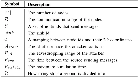
TABLE I: Model parameters
Symbol Description
|V| The number of nodes
R The communication range of the nodes
S A set of node ids that send messages
sink The sink id
C A mapping between node ids and their 2D coordinates
Astart The id of the node the attacker starts at
RA The eavesdropping range of the attacker
Psrc The time between the source sending messages
Psaf ety The maximum simulation time
Ω How many slots a second is divided into
locations [23], (ii) energy efficient routing [24], and (iii) others [25], is constraint programming (CP). CP is a type of programming described using a set of decision variables that store the output of the model, an objective function that ranks the goodness of variables and a set of constraints that define what values for a solution are valid. Using a solver, an optimal solution for the problem can be obtained.
Similar to CP, is integer linear programming (ILP) where the relations specified in the constraints between the variables must be linear. ILP has been used to find solutions that optimise for energy usage or delivery latency in a WSN. Our approach will instead optimise the routing of messages to provide SLP.
III. CONSTRAINTPROGRAMMINGMODEL
In this section we describe the ILP model1, including the
rationale for certain constraints. Our ILP model is written in IBM’s Optimisation Programming Language (OPL). There are multiple ILP solvers present with IBM ILOG CPLEX version 12.6.3. We used the CP solver as it was able to produce optimal results faster and also scale to larger network sizes than the CPLEX solver. The CP solver proves optimality by showing that no better solution can be found, while the CPLEX solver
obtains a lower bound proof using cuts and linear relaxation.2
The network was modelled as a directed graph G= (V, A)
whereV is the set of nodes andAis the set of arcs. An arc is
a 2-tuple(u, v)whereuis the origin andv is the target. Each
node inV was assigned a 2D coordinate C and the euclidean
distance was calculated between each node. If the distance between two different nodes was less than or equal to the
communication rangeRof the sensor nodes, then that arc is
present inA. By using a directional graph we can model more
networks, in this work if (u, v) ∈A =⇒ (v, u)∈ A. The
paths that messages can travel along is defined by the arcs in
Athen and the paths the attacker can move along is modelled
as a directed graphGA= (V, AA) routed at the node with id
Astart where the attacker starts. If the distance between two
nodes is less than the attacker’s eavesdropping rangeRAthen
AA contains that arc, this also means the attacker can move
along that arc. Once the attacker finds the source it will remain
1The source code for this model can be found at bitbucket.org/MBradbury/
slp-attacker-ilp/raw/a4e326e/SLP/SLP.mod
at that location, so the attacker cannot move along arcs which start at the source. As the attacker moves through the network, it can only move to be co-located with another node. In this paper, we assume the attacker’s eavesdropping range is equal
to the sensor node’s transmission range (R=RA).
The sink is a special node to which messages are routed
and the sources (S) are nodes that generate one message every
Psrc. We assume there is a single sink and source.
There is an upper bound on the duration of the model (Psaf ety), within which routing and attacker movement is
considered. Time (T) is discretised by dividing it into slots,
there are Ω slots per second. Each node can send a single
message in each slot. A node may choose to send no messages in a given slot. The attacker can therefore either move in response to a single message or not move at all in a given slot. To ensure the attacker could reach the source, the attacker’s starting position was never set so its distance in hops from
the source was greater than Psrc·Ω. As otherwise the safety
period may be reached before the attacker has a chance to capture the source. The attacker can respond to a message a neighbour sends in a time slot if that message had not been previously responded to. If no messages are sent by a neighbour the attacker must remain where it is.
Time 0 is special as it is used to set the attacker’s position, no messages are sent at this time. After time 0 when a node broadcasts a message we assume network links are perfect and all neighbours receive the message, even if multiple nodes broadcast in that time slot. In this case we assume a collision detection and retransmission is used to ensure message delivery.
Messages generated by a source (M) are represented by a
2-tuple where the first element (src) is the id of the source that generated the message and the second element (seq) is the message number. This ensures each message is unique.
\
Psaf ety=dΩ·Psaf etye (1)
d
Psrc=dΩ·Psrce (2)
T = 0..Psaf ety\ (3)
T1= 1..Psaf ety\ (4)
M= {(src, seq)|src∈ S,
seq∈1..dPsaf ety·Psrce }
(5)
D(i, j) =p(i.x−j.x)2+ (i.y−j.y)2 (6)
A={(u, v)|u, v∈V, D(u, v)≤ R ∧u6=v} (7)
N(i) ={j|(i, j)∈A, i6=j} (8)
AA={(u, v)|u, v∈V, D(u, v)≤ RA} \
{(s, v)|s∈ S, v∈V, s6=v} (9)
NA(i) ={j|(i, j)∈AA, i6=j} (10)
A. Objective Function
Two decision variables are used to capture the output of the model. The broadcasts performed is a three dimensional array of booleans with the node ids, message and time as the dimensions (B:V × M × T →B). This variable is intended to capture
whether a node sends a message at a given time. The other
decision variable is the attacker path which is a two dimensional array of booleans with time and the arcs an attacker can take
as the dimensions (PA:T ×AA→B). This variable captures
whether at a given time an attacker moves along an arc. The objective function for this model is to maximise the distance between the attacker’s final position and the source(s) in the network. As the aim in providing SLP is to prevent the attacker from reaching the source, we can say the further the attacker is from the source the better SLP has been provided within a safety period.
maximise X
s∈S
e∈AA
PA(P\saf ety, e)·D(s, e.v)
subject to Routing Constraints ctR1 to ctR6,
Attacker Constraints ctA1 to ctA7. (11)
B. Routing Constraints
Here, the constraints on how messages are generated by the source and how they are routed in the network are described.
ctR1 Att= 0, no messages are broadcasted.
ctR2 Fromt >0, each source node generates a message every
Psrc until the safety period is reached.
ctR3 No node can broadcast more that a single message
concurrently. This means that in a given time slot a node must send one message or no messages.
ctR4 Once a message is broadcasted by a node it is not
broadcasted by that node again.
ctR5 A node can only forward a message after a neighbour
broadcasted that message in a previous time slot.
ctR6 All messages sent by the sources must reach the sink.
∀n∈V •∀m∈ M•B(n, m,0) = 0 (ctR1)
∀n∈ S•∀m∈ M:m.src=n•
B(n, m,(m.seq−1)·Pdsrc+ 1)
(ctR2)
∀τ ∈ T1•∀n∈V •1≥ X
m∈M
B(n, m, τ) (ctR3)
∀m∈ M•∀n∈V •∀τ1∈ T1•
B(n, m, τ1) =⇒ 0 =
X
τ2∈T, τ2>τ1
B(n, m, τ2) (ctR4)
∀n∈(V \ S)•∀m∈ M•∀τ1∈ T1•
B(n, m, τ1) =⇒ 1≤
X
neigh∈N(n)
τ2∈T,0<τ2<τ1
B(neigh, m, τ2) (ctR5)
∀m∈ M•1≤X
n∈N(sink)
τ∈T1
B(n, m, τ) (ctR6)
C. Attacker Constraints
in response to messages (ctA4, ctA7) and (ii) the attacker will only consider a message once as otherwise it might follow that message as it moves away from the source (ctA5, ctA6).
To simplify attacker constraints four predicates about the
attacker’s movement are defined. AM2Achecks if the attacker
moved to n at timeτ. AM2NAchecks if the attacker moved
to a neighbour ofnatτ.ASMchecks if the attacker remained
where it was atτ.AMBAchecks if an attacker moved because
of a message matτ.
AM2A(n, τ) = 1 =X
e∈AA, e.v=n
PA(τ, e) (12)
AM2NA(n, τ) = 1 =X
neigh∈NA(n)
AM2A(neigh, τ) (13)
ASM(τ) = 1 =X
e∈AA, e.u=e.v
PA(τ, e) (14)
AMBA(m, τ) = 1 =X
e∈AA, e.u6=e.v
PA(τ, e)∧B(e.v, m, τ) (15)
ctA1 Att= 0 the attacker moves from the attacker’s starting
position to that same position.
ctA2 The attacker makes exactly one move each time slot.
ctA3 A move must be from the attacker’s current location.
ctA4 If the attacker moves tonfrommat timeτ, then it must
be because at time τ the nodenbroadcasted a message.
ctA5 If the attacker receives a message that it has not
previously moved in response to, then the attacker moves in response to that message.
ctA6 If the attacker moved in response to a message at timeτ,
then at no timeτ0 > τ will the attacker move in response
to that message again.
ctA7 If the attacker is at node nand no neighbours send a
message, then the attacker moves along the (n,n) edge.
PA(0,(Astart,Astart)) = 1 (ctA1)
∀τ ∈ T •1 =X
e∈AA
PA(τ, e) (ctA2)
∀τ ∈ T1•1 = X
e1,e2∈AA, e1.v=e2.u
PA(τ−1, e1)∧PA(τ, e2) (ctA3)
∀n∈V •∀τ ∈ T1•
1 =X
e∈AA, e.v=n∧e.u6=e.v
PA(τ, e) =⇒ 1 =
X
m∈M
B(n, m, τ) (ctA4)
∀n∈V •∀m∈ M•∀τ ∈ T1•
B(n, m, τ)∧AM2NA(n, τ −1)∧0 =X
t2∈T,0<τ2<τ
AMBA(m, τ2)
=⇒ AM2A(n, τ) (ctA5)
∀τ1∈ T1•∀m∈ M•
AMBA(m, τ1) =⇒ 0 =
X
τ2∈T, τ2>τ1
AMBA(m, τ2) (ctA6)
∀τ ∈ T1•∀e∈AA•
PA(τ−1, e)∧0 =
X
n∈NA(e.v)
m∈M
B(n, m, τ) =⇒ ASM(τ)
(ctA7)
IV. MODELRESULTS
In this section we describe the output from the ILP model
for one combination of parameters3. We ran the model for
a variety of different parameters including 3x3, 4x4 and 5x5 grids with the sink and source at different locations. Larger networks became infeasible to run due to the large amount of memory required. The results in Figure 1 show a 5x5 network with the source in the top left corner and the attacker starting at the sink which was positioned in the centre. This configuration was chosen as it has been previously investigated [9, 10] and allowed the state space of the model to be small enough for a solution to be found within a reasonable time.
Figures 1a to 1g show the pattern of broadcasts and Figure 1h shows how the distance of the attacker from the source changes over time. From the results we observed four major trends:
1) The routing path should go around the sink and approach from the opposite direction to the source.
2) Some routes should take the shortest path from the source to the sink.
3) Messages should be delayed so multiple messages are grouped together.
4) Messages should be delayed as late as possible with respect to the safety period.
Some of these observations have been used in previous work, while others have not. For example, having the route approach the sink from a direction other than the one the source is in has been used in Phantom Routing [3] and Ring-based Routing [7]. We have also seen algorithms whose routes occasionally take the shortest path [26]. However, we have not seen delaying and grouping messages previously in providing SLP. By delaying and grouping messages the attacker should end up with less time to make moves towards the sink within the safety period as shown by Figure 1h, where the attacker moves mainly near the end of the simulation (towards the top of the graph). By grouping and allowing messages to be delivered out-of-order we also force the attacker to require a larger memory to ensure previously received messages are ignored in the future.
V. ROUTINGALGORITHM
In this section we describe the implementation of the routing algorithm inspired by the model’s output. There are four stages: 1) AvoidSink: In this first stage messages are routed around
the sink.
2) Backtrack: Messages may end up attempting to go towards the sink and not having any valid routes, so they need to backtrack.
3) ToSink: Once a message has finished routing to avoid the sink it needs to be delivered to the sink.
4) FromSink: Finally, the message is sent in a starburst from the sink.
A. Stage 1: Avoid Sink
In order to provide SLP the most important thing we need to do is be able to route messages reliably around the sink and have
(a) Message 1 1 1 42 42 50 50 51 51 54 55 55 59 59 63 63 63
1 2 3 4 5
6 7 8 9 10
11 12 13 14 15
16 17 18 19 20
21 22 23 24 25
(b) Message 2
10 10 32 32 36 36 40 40 41 46 46 50 50 52 52 53 53 54 54 60 61 61 62 62 62
1 2 3 4 5
6 7 8 9 10
11 12 13 14 15
16 17 18 19 20
21 22 23 24 25
(c) Message 3
19 19 46 46 54 54 54 55 55 55 57 57 57 62 62
1 2 3 4 5
6 7 8 9 10
11 12 13 14 15
16 17 18 19 20
21 22 23 24 25
(d) Message 4
28 28 52 52 53 53 53 54 54 54
1 2 3 4 5
6 7 8 9 10
11 12 13 14 15
16 17 18 19 20
21 22 23 24 25
(e) Message 5
37 37 46 46 47 47 50 50 52 56 56 57 57 58 58 58
1 2 3 4 5
6 7 8 9 10
11 12 13 14 15
16 17 18 19 20
21 22 23 24 25
(f) Message 6
46 46 51 51 52 52 53 53 54 54 54 56 56 56 57 57 57 61 61 62
1 2 3 4 5
6 7 8 9 10
11 12 13 14 15
16 17 18 19 20
21 22 23 24 25
(g) Message 7
55 55 57 57 58 58 59 59 59 60 60 60
1 2 3 4 5
6 7 8 9 10
11 12 13 14 15
16 17 18 19 20
21 22 23 24 25
[image:6.612.58.567.45.317.2](h) Attacker Distance from Source
Fig. 1: An output of the ILP model for a 5x5 network with node 1 sending 7 messages to the sink at node 13 with a period of 1 second and 1 second is broken up into 9 slots. The attacker starts at node 13. Message broadcasts are represented by arrows from the sending node to the receiving nodes, the arrows are labelled with the time slot of the broadcast. Lines in (h) are labelled with the message number the attacker responded to and the location of the attacker is shown above the point.
them approach it from the opposite direction that the source is in. This requires every node to be aware of its neighbours, as one will be chosen to be the next in the path. We also require
that every nodenknows its distance to the sink ∆sink(n), its
distance from the source∆src(n)and the distance between the
sink and source ∆ss. These values are found by the landmark
nodes (sink/source) flooding the network. Every node should know these values for each node in its 1-hop neighbourhood.
There is a parameter called message group size which
specifies how many messages to group together. By grouping together the algorithm will delay the messages each hop so
that the messages reach ∆ss hops travelled at the same time.
Messages sent earlier in the group will be delayed longer. The
delay is specified in Equation 16, where i is the position in
the message group,Psrc is the source period andαis the time
it takes a message to send from one node to another. This is calculated at the source when the message is sent.
delay(i) = i·Psrc+α·∆ss
∆ss
(16)
Retransmissions are used to ensure reliability along the route. If retransmissions to a target fail a fixed number of times, then that target is blacklisted and another node will attempt to be used. If further retransmissions fail, then a poll message is sent which asks neighbours to broadcast their information. This is performed to ensure that the most up-to-date information is being used to make the routing decisions. Retransmissions are stopped when an acknowledgement packet is received or the maximum number of retransmissions have been sent.
0 1 2 3 4 5 6 7 8
9 10 11 12 13 14 15 16 17
18 19 20 21 22 23 24 25 26
27 28 29 30 31 32 33 34 35
36 37 38 39 40 41 42 43 44
45 46 47 48 49 50 51 52 53
Fig. 2: Showing the links a nodenhas between eachm
neigh-bour in its one hop neighneigh-bourhood that satisfies:∆src(m)>
∆src(n)∧ ∆sink(n)>∆ss2 ∨∆sink(m)≥∆sink(n)
. Nodes that have no neighbours that satisfy this are marked in gray. The source is a pentagon and the sink is a hexagon.
B. Stage 2: Backtrack
There is the possibility that a message may reach a node which has no further neighbours to choose from, for example node 20 in Figure 2. In this case the message backtracks to a node that is further from the sink that was not the previous hop in the route. The next hop is then chosen using the avoid sink logic. This should allow a message to avoid the area of nodes that should not be used in the routing path (highlighted in
grey in Figure 2). Backtracking is only done on noden when
∆src(n)<∆ssas this is a node that would otherwise lead the
[image:6.612.357.519.379.500.2]C. Stage 3: To Sink
When a node’s∆src(n)≥∆ssthen the message has passed the
area that would lead it towards the source. When this message has reached a node with no neighbours that are further from the sink, the message is at a local maxima for the sink distance, so the message is routed back towards the sink. When a message reaches a certain number of hops travelled it is routed back to the sink. This is to ensure bounded message latency and to prevent the message going too far on very large networks. As with routing to avoid the sink, retransmissions and blacklisting are used to provide a reliable message transmission to the sink.
D. Stage 4: From Sink
Finally, once the message reaches the sink, it is broadcasted in a starburst pattern away from the sink in all directions for a limited number of hops. Model results where the sink was the furthest point required this behaviour to ensure that the attacker is lured to the furthest location from the source. This behaviour was also observed in Figure 1g.
VI. EXPERIMENTALSETUP
A. Simulation Environment and Network Configuration
The TOSSIM (V2.1.2) simulation environment was used in all experiments [27]. TOSSIM is a discrete event simulator capable of accurately modelling sensor nodes and the modes of communications between them.
A square grid network layout of size n×n was used in
all experiments, where n ∈ {11,15,21,25}, i.e., networks
with 121, 225, 441 and 625 nodes respectively. The node
neighbourhoods were generating using LinkLayerModel4 with
the parameters in [10, Table I]. Noise models were created
using the first 2500 lines of casino-lab.txt5. A single
source node generated messages and a single sink node collected messages. These nodes were assigned positions in the SourceCorner configuration from [9], where the source is in the top left corner and the sink at the centre of the grid. The rate at which messages from the real source were generated was varied, as shown in Section VII. At least 10,000 repeats were performed for each combination of parameters. Nodes were located 4.5 meters apart. The node separation distance was determined experimentally, based on observing the pattern of transmissions in the simulator. This separation distance ensured that messages (i) pass through multiple nodes from source to sink, (ii) can move only one hop at a time, and (iii) will usually only be passed to horizontally or vertically adjacent nodes.
B. Attacker Model
A reactive attacker model based on the patient adversary introduced in [3] is used. The attacker initially starts at the sink. When a message is received the attacker will move to the 1-hop source’s location if that message has not been received before. To detect if a message has been received before, we
4LinkLayerModel is a tool provided with TOSSIM that extrapolates link
strengths from node coordinates based on experimental data.
[image:7.612.346.529.71.141.2]5casino-lab.txt is a noise sample file provided with TOSSIM.
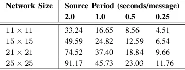
TABLE II: Safety Period (seconds).
Network Size Source Period (seconds/message)
2.0 1.0 0.5 0.25
11×11 33.24 16.65 8.56 4.51
15×15 49.59 24.82 12.59 6.54
21×21 74.52 37.40 18.84 9.66
25×25 91.17 45.73 23.03 11.76
assume that an attacker has access to the message type and sequence number. Once the source has been found the attacker will no longer move. This is commensurate with the attacker models used in [8, 9, 10].
C. Safety Period
A metric called safety period was introduced in [3] which
captured the number of messages needed to capture the source. The higher the safety period is, the higher is the privacy level. This issue with this definition of safety period is that it is unbounded and in problem of asset monitoring it does not make sense to consider an unbounded safety period.
If the asset is immobile, then the attacker can simply perform an exhaustive search of the network and providing SLP is irrelevant. If the asset is mobile, then performing an exhaustive search is less desirable as an asset may move into a previously searched area of the network. So using the context provided by message broadcasts is preferred. This means that the SLP
problem can only be considered when it istime-bounded, i.e.,
when the asset has to be captured within a certain time window.
Therefore, we use an alternate by analogous definition ofsafety
period, where if the attacker fails to capture the source within this period it is considered to have failed to capture the source.
As flooding has been shown to provide no SLP [3] we use the average time it takes the attacker to capture the source as a baseline and double it to calculate the safety period (shown in table II) for the protocol in this paper.
D. Simulation Experiments
An experiment constituted a single execution of the simulation environment using a specified protocol configuration, network size and safety period. An experiment terminated when the source node had been captured or the safety period had expired. An attacker was implemented based on the log output from TOSSIM. It maintains internal state about its location using node identifiers. When a node receives a message, if the attacker is at that location it will move based on the attacker model.
The algorithm being tested has four parameters: the max-imum walk length, the buffer size, the number of messages to group and the probability the message is sent directly to the sink. As the maximum walk length is simply to provide a finite bound in large networks, it was set to 100 hops. The
number of messages to group was varied between{1, 2, 3, 4}.
The buffer size was set to 10 messages as we do not expect more than 10 concurrent messages being sent in the network at one time. Finally, the probability of sending a message directly
Msg Group Size 1 Msg Group Size 2 Msg Group Size 3 Msg Group Size 4 0 20 40 60 80 100
11 15 21 25
R e ce iv e R a ti o ( % ) Network Size
(a) Source Period 2.0 seconds
0 20 40 60 80 100
11 15 21 25
R e ce iv e R a ti o ( % ) Network Size
[image:8.612.46.571.50.278.2](b) Source Period 0.25 seconds
Fig. 3: Results showing the receive ratio.
Msg Group Size 1 Msg Group Size 2 Msg Group Size 3 Msg Group Size 4
0 1 2 3 4 5 6 7 8 9
11 15 21 25
C a p tu re R a ti o ( % ) Network Size
(a) Source Period 2.0 seconds
0 1 2 3 4 5 6 7 8 9
11 15 21 25
C a p tu re R a ti o ( % ) Network Size
(b) Source Period 0.25 seconds
Fig. 4: Results showing the capture ratio.
VII. RESULTS
As part of these results we will analyse four key metrics: (i)
receive ratio: the percentage of messages sent by the source
and received at the sink, (ii) capture ratio: the percentage of
runs in which the source was captured, (iii) messages sent
per second: the number of messages sent by all nodes in
the network per second, and (iv) latency: the time it takes a
message sent by the source to be received at the sink. All results shown are for when the probability that a message is sent directly to the sink is 20%. Lower probabilities gave similar, but slightly worse results and higher probabilities produced much worse results. Therefore, for reasons of space, we have omitted results for the probabilities of 0%, 40% and 60% as 20% performed better. Also, only the results for the two source periods 2 and 0.25 seconds per message are included as the patterns between these are similar to the results for 1 and 0.5 seconds per message.
A. Receive Ratio
A high receive ratio between 75% and 95% is observed. Fewer messages were delivered with larger networks and larger messages group sizes. This suggests that the attacker was hearing most of the source messages, meaning that the privacy level imparted by the algorithm is due to the efficiency of the protocol and not due to the unreliability of the network.
B. Capture Ratio
There is a less than 10% probability of the attacker capturing the source within the safety period for these parameter combinations. As more messages are grouped together, the capture ratio falls lower. This matches with our previous intuition that a greater number of messages grouped together would give the attacker fewer chances to respond to messages within the safety period. On the other hand, with messages
Msg Group Size 1 Msg Group Size 2 Msg Group Size 3 Msg Group Size 4
0 50 100 150 200 250 300
11 15 21 25
T o ta l M e ss a g e s S e n t p e r S e co n d Network Size
(a) Source Period 2.0 seconds
0 50 100 150 200 250 300
11 15 21 25
T o ta l M e ss a g e s S e n t p e r S e co n d Network Size
(b) Source Period 0.25 seconds
Fig. 5: Results showing the messages sent per second.
Msg Group Size 1 Msg Group Size 2 Msg Group Size 3 Msg Group Size 4
0 500 1000 1500 2000 2500 3000 3500 4000
11 15 21 25
N o rm a l M e ss a g e L a te n cy ( m s) Network Size
(a) Source Period 2.0 seconds
0 500 1000 1500 2000 2500 3000 3500 4000
11 15 21 25
N o rm a l M e ss a g e L a te n cy ( m s) Network Size
(b) Source Period 0.25 seconds
Fig. 6: Results showing the message latency.
being grouped together, it suggests that the message delivery latency may be increased. When the size of the message group is high, the protocol delivers near optimal privacy level.
As has been previously observed in [9, 10], we also see that larger networks tend to have lower capture ratios.
C. Messages Sent per Second
As the different network sizes being varied each has a different safety period, the number of messages sent has been normalised with respect to the simulation length to allow the results to be compared. The results show that the number of messages sent does not vary greatly for different numbers of messages to group together. For faster message rates, larger message group sizes require slightly fewer messages sent per second.
D. Latency
The longer the time between messages, the larger the latency between a source sending the message and the sink receiving the message. This is because messages are delayed to make sure that the number requested are about the sink-source distance from the source. When there are multiple messages the per hop delay needs to be longer. These results indicate that there is a trade off between latency and capture ratio, to obtain a better capture ratio using this technique a larger latency will be required. For many applications a latency of this magnitude will be acceptable. For example tracking the location of a slow moving panda will not be adversely affected. But in scenarios where very low latency is important, such as on a battlefield, this technique may be less suitable.
VIII. DISCUSSION
within the safety period. Attempting to optimise this model for other objective functions such as minimising latency or the total number of messages sent might produce different output indicating other kinds of routing that would provide SLP.
IX. CONCLUSION
In this paper we have presented a novel formalisation of SLP-aware routing as an ILP constraint satisfaction problem. This model produced optimal routes computed based on global network knowledge, making these routes unamenable to deployment. We then presented a distributed routing protocol inspired by the optimal solution and performed large scale simulations to judge the performance. Our results show that we can obtain low capture ratios (high levels of SLP) with the tradeoff being a higher delivery latency. For future work we aim to expand the model to include fake message broadcasts and to also look at optimising for other objective functions such as the number of messages sent and the delivery latency.
ACKNOWLEDGEMENTS
This research was supported the Engineering and Physical Sci-ences Research Council (EPSRC) [DTG grant EP/M506679/1].
REFERENCES
[1] A. Mainwaring, D. Culler, J. Polastre, R. Szewczyk, and J. Anderson, “Wireless sensor networks for habitat monitoring,”
in Proceedings of the 1st ACM International Workshop on
Wireless Sensor Networks and Applications, ser. WSNA ’02.
New York, NY, USA: ACM, 2002, pp. 88–97.
[2] A.-M. Badescu and L. Cotofana, “A wireless sensor network to monitor and protect tigers in the wild,”Ecological Indicators, vol. 57, pp. 447–451, 2015.
[3] P. Kamat, Y. Zhang, W. Trappe, and C. Ozturk, “Enhancing source-location privacy in sensor network routing,” in25thIEEE International Conference on Distributed Computing Systems
(ICDCS’05), Jun. 2005, pp. 599–608.
[4] C. Ozturk, Y. Zhang, and W. Trappe, “Source-location privacy in energy-constrained sensor network routing,” inProceedings
of the 2nd ACM workshop on Security of ad hoc and sensor
networks, ser. SASN ’04. New York, NY, USA: ACM, 2004,
pp. 88–93.
[5] M. Conti, J. Willemsen, and B. Crispo, “Providing source location privacy in wireless sensor networks: A survey,”IEEE
Communications Surveys and Tutorials, vol. 15, no. 3, pp. 1238–
1280, 2013.
[6] P. Spachos, D. Toumpakaris, and D. Hatzinakos, “Angle-based dynamic routing scheme for source location privacy in wireless sensor networks,” in Vehicular Technology Conference (VTC
Spring), 2014 IEEE 79th, May 2014, pp. 1–5.
[7] L. Yao, L. Kang, F. Deng, J. Deng, and G. Wu, “Protecting source–location privacy based on multirings in wireless sen-sor networks,” Concurrency and Computation: Practice and
Experience, vol. 27, no. 15, pp. 3863–3876, 2015.
[8] A. Jhumka, M. Leeke, and S. Shrestha, “On the use of fake sources for source location privacy: Trade-offs between energy and privacy,”The Computer Journal, vol. 54, no. 6, pp. 860–874, 2011.
[9] A. Jhumka, M. Bradbury, and M. Leeke, “Fake source-based source location privacy in wireless sensor networks,”
Concur-rency and Computation: Practice and Experience, vol. 27, no. 12,
pp. 2999–3020, 2015.
[10] M. Bradbury, M. Leeke, and A. Jhumka, “A dynamic fake source algorithm for source location privacy in wireless sensor networks,”
in14thIEEE International Conference on Trust, Security and
Privacy in Computing and Communications (TrustCom), Aug.
2015, pp. 531–538.
[11] J. Long, M. Dong, K. Ota, and A. Liu, “Achieving source location privacy and network lifetime maximization through tree-based diversionary routing in wireless sensor networks,”IEEE Access, vol. 2, pp. 633–651, 2014.
[12] W. Tan, K. Xu, and D. Wang, “An anti-tracking source-location privacy protection protocol in WSNs based on path extension,”
Internet of Things Journal, IEEE, vol. 1, no. 5, pp. 461–471,
Oct. 2014.
[13] M. Dong, K. Ota, and A. Liu, “Preserving source-location privacy through redundant fog loop for wireless sensor networks,” in
13th IEEE International Conference on Dependable, Autonomic
and Secure Computing (DASC), Liverpool, UK, Oct. 2015, pp.
1835–1842.
[14] M. Mahmoud and X. Shen, “A cloud-based scheme for protecting source-location privacy against hotspot-locating attack in wireless sensor networks,” Parallel and Distributed Systems, IEEE
Transactions on, vol. 23, no. 10, pp. 1805–1818, Oct. 2012.
[15] M. Shao, W. Hu, S. Zhu, G. Cao, S. Krishnamurth, and T. La Porta, “Cross-layer enhanced source location privacy in sensor networks,” in6thAnnual IEEE Communications Society Conference on Sensor, Mesh and Ad Hoc Communications and
Networks (SECON ’09), 2009, pp. 1–9.
[16] S. Oh and M. Gruteser, “Multi-node coordinated jamming for location privacy protection,” inMilitary Communications
Conference (MILCOM), 2011 IEEE, Nov. 2011, pp. 1243–1249.
[17] M. Raj, N. Li, D. Liu, M. Wright, and S. K. Das, “Using data mules to preserve source location privacy in wireless sensor networks,”Pervasive and Mobile Computing, vol. 11, pp. 244– 260, 2014.
[18] J. P. Singh, P. K. Roy, S. K. Singh, and P. Kumar, “Source location privacy using data mules in wireless sensor networks,”
in2016 IEEE Region 10 Conference (TENCON), Nov. 2016, pp.
2743–2747.
[19] Z. Benenson, P. M. Cholewinski, and F. C. Freiling,Wireless
Sensors Networks Security. IOS Press, 2008, ch. Vulnerabilities
and Attacks in Wireless Sensor Networks, pp. 22–43.
[20] K. Mehta, D. Liu, and M. Wright, “Protecting location privacy in sensor networks against a global eavesdropper,”IEEE Trans.
on Mobile Computing, vol. 11, no. 2, pp. 320–336, Feb. 2012.
[21] Y. Yang, M. Shao, S. Zhu, and G. Cao, “Towards statistically strong source anonymity for sensor networks,”ACM Trans. Sen.
Netw., vol. 9, no. 3, pp. 34:1–34:23, Jun. 2013.
[22] A. Proa˜no, L. Lazos, and M. Krunz, “Traffic decorrelation techniques for countering a global eavesdropper in WSNs,”IEEE
Trans. on Mobile Computing, vol. 16, no. 3, pp. 857–871, Mar.
2017.
[23] A. Boubrima, W. Bechkit, and H. Rivano, “Optimal WSN deploy-ment models for air pollution monitoring,”IEEE Transactions
on Wireless Communications, vol. PP, no. 99, pp. 1–1, 2017.
[24] J.-H. Chang and L. Tassiulas, “Maximum lifetime routing in wireless sensor networks,” IEEE/ACM Transactions on
Networking, vol. 12, no. 4, pp. 609–619, Aug. 2004.
[25] R. Asorey-Cacheda, A.-J. Garcia-Sanchez, F. Garcia-Sanchez, and J. Garcia-Haro, “A survey on non-linear optimization problems in wireless sensor networks,”Journal of Network and
Computer Applications, vol. 82, pp. 1–20, 2017.
[26] C. Gu, M. Bradbury, and A. Jhumka, “Phantom walkabouts in wireless sensor networks,” in Proceedings of the 2017 ACM
Symposium on Applied Computing, ser. SAC’17. New York,
NY, USA: ACM, Apr. 2017, pp. 609–617.
[27] P. Levis, N. Lee, M. Welsh, and D. Culler, “Tossim: accurate and scalable simulation of entire tinyos applications,” inProceedings
of the 1st international conference on Embedded networked
sensor systems, ser. SenSys ’03. New York, NY, USA: ACM,