Faster exponential time algorithms in graphs of bounded average degree

(1)

http://wrap.warwick.ac.uk/

Original citation:

Cygan, Marek and Pilipczuk, Marcin. (2013) Faster exponential-time algorithms in

graphs of bounded average degree. Information and Computation . ISSN 0890-5401 (In

Press)

Permanent WRAP url:

http://wrap.warwick.ac.uk/66081

Copyright and reuse:

The Warwick Research Archive Portal (WRAP) makes this work of researchers of the

University of Warwick available open access under the following conditions. Copyright ©

and all moral rights to the version of the paper presented here belong to the individual

author(s) and/or other copyright owners. To the extent reasonable and practicable the

material made available in WRAP has been checked for eligibility before being made

available.

Copies of full items can be used for personal research or study, educational, or

not-for-profit purposes without prior permission or charge. Provided that the authors, title and

full bibliographic details are credited, a hyperlink and/or URL is given for the original

metadata page and the content is not changed in any way.

Publisher statement:

NOTICE: this is the author’s version of a work that was accepted for publication in

Information and Computation. Changes resulting from the publishing process, such as

peer review, editing, corrections, structural formatting, and other quality control

mechanisms may not be reflected in this document. Changes may have been made to

this work since it was submitted for publication. A definitive version was subsequently

published in http://dx.doi.org/10.1016/j.ic.2014.12.007

A note on versions:

The version presented here may differ from the published version or, version of record, if

you wish to cite this item you are advised to consult the publisher’s version. Please see

the ‘permanent WRAP url’ above for details on accessing the published version and note

that access may require a subscription.

(2)

Faster exponential-time algorithms in graphs of bounded average degree

I

Marek Cygana, Marcin Pilipczuka

a_{Institute of Informatics, University of Warsaw, Poland}

Abstract

We present a number of exponential-time algorithms for problems in sparse matrices and graphs of bounded average degree. First, we obtain a simple algorithm that computes a permanent of ann×nmatrix over an arbitrary commutative ring with at mostdnnon-zero entries usingO?(2(1−1/(3.55d))n_{) time and ring operations}1_{, improving and simplifying}

the recent result of Izumi and Wadayama [FOCS 2012].

Second, we present a simple algorithm for counting perfect matchings in ann-vertex graph inO?(2n/2_{) time and}

polynomial space; our algorithm matches the complexity bounds of the algorithm of Bj¨orklund [SODA 2012], but relies on inclusion-exclusion principle instead of algebraic transformations.

Third, we show a combinatorial lemma that bounds the number of “Hamiltonian-like” structures in a graph of bounded average degree. Using this result, we show that

1. a minimum weight Hamiltonian cycle in ann-vertex graph with average degree bounded bydcan be found in O?(2(1−εd)n_{) time and exponential space for a constant}ε

ddepending only ond;

2. the number of perfect matchings in ann-vertex graph with average degree bounded bydcan be computed in O?(2(1−ε0d)n/2) time and exponential space, for a constantε0

ddepending only ond.

The algorithm for minimum weight Hamiltonian cycle generalizes the recent results of Bj¨orklund et al. [TALG 2012] on graphs of bounded degree.

Keywords: moderately-exponential algorithms, bounded average degree, counting perfect matchings, minimum weight Hamiltonian cycle

1. Introduction

Improving upon the 50-years oldO?(2n_{)-time dynamic programming algorithms for the Traveling Salesman}

Prob-lem by Bellman [1] and Held and Karp [2] is a major open probProb-lem in the field of exponential-time algorithms [3]. A similar situation appears when we want to count perfect matchings in a graph: a half-century oldO?(2n/2_)-time

algorithm of Ryser for bipartite graphs [4] has only recently been transferred to arbitrary graphs [5], and breaking these time complexity barriers seems like a very challenging task.

From a broader perspective, improving upon a trivial brute-force or a simple dynamic programming algorithm is one of the main goals of the field of exponential-time algorithms. The last few years brought a number of positive results in that direction, most notably the O?(1.66n) randomized algorithm for finding a Hamiltonian cycle in an undirected graph [6]. However, it is conjectured (the so-called Strong Exponential Time Hypothesis [7]) that the central problem of satisfying a general CNF-SAT formulae does not admit any exponentially better algorithm than the trivial brute-force one. A number of lower bounds were proven using this assumption [8, 9, 10].

Although the aforementioned 2n_{or 2}n/2_{-barriers may be di}_ffi_{cult or even outright impossible to break, it seems}

reasonable to suspect that additional assumptions on the graph structure, such as bounded degree or bounded average

1_The_O?_{-notation suppresses factors polynomial in the input size.}

I_{A preliminary version of this work has been presented at ICALP 2013.}

(3)

degree, simplify the computational tasks significantly. In the case of the problem of counting perfect matchings in bipartite graphs, the classic algorithm of Ryser [4] the best known improvement in general graphs is an algorithm running in expected timeO?(2(1−O(n2/3_log_n))_·_n_/₂

) due to Bax and Franklin [11]. If one assumes bounded average degree, faster algorithms have been given by Servedio and Wan [12] and, very recently, by Izumi and Wadayama [13]. In Section 2 we continue this line of research and show the following.

Theorem 1. For any commutative semiring R, given an m×n matrix M, m≤n with elements from R with at most dm non-zero entries for some d ≥2, one can compute the permanent of M usingO?(2(1−1/(3.55d))m)time and performing O?(2(1−1/(3.55d))m)operations over the semiring R. The algorithm may require to use exponential space and store an exponential number of elements from R.

Note that the number of perfect matchings in a bipartite graph is equal to the permanent of the adjacency matrix of this graph (computed over_Z). Hence, we improve the running time of [13, 12] in terms of the dependency ond. We would like to emphasise that our proof of Theorem 1 is elementary and does not need the advanced techniques of coding theory used in [13].

Since the algorithm of Theorem 1 is able to handle the computation of the permanent of any matrix over commu-tative semiring, not only the special case of computing the number of perfect matchings, our result shows also that the running time of the algorithm of Bj¨orklund et al. [14] can be improved for sparse matrices.

In Section 3, we move to the problem of counting perfect matchings in general graphs. An algorithm solving this problem inO?(2n/2_{) time, that is, in time matching the bound for bipartite graphs, has been discovered very recently,}

in 2012, by Bj¨orklund [5]. Bj¨orklund’s result improved upon previous algorithms with running timeO?(1.732n_{) due}

to Bj¨orklund and Husfeldt [15] and with running timeO?(1.619n) due to Koivisto [16]. We remark that, in contrast, the corresponding algorithm of Ryser [4] for bipartite graphs is already 50-years old. In Section 3, we observe that the problem of counting perfect matchings in general graphs can be reduced to a problem of counting some special types of cycle covers, which, in turn, can be done inO?(2n/2)-time and polynomial space for ann-vertex graph, using the inclusion-exclusion principle. Thus, we obtain a new proof of the main result of [5], using the inclusion-exclusion principle instead of advanced algebraic transformations.

The problem of counting some special types of cycle covers, introduced in Section 3, moves us to the area of Hamiltonian-like problems. In 2008 Bj¨orklund et al. [17] observed that the classic dynamic programming algorithm for finding minimum weight Hamiltonian cycle can be trimmed to running timeO?(2(1−ε∆)n_{) in graphs of maximum}

degree∆. The cost of this improvement is the use of exponential space, as we can no longer easily translate the dynamic programming algorithm into an inclusion-exclusion formula. The ideas from [17] were also applied to the Fast Subset Convolution algorithm [18], yielding a similar improvements for the problem of computing the chromatic number in graphs of bounded degree [19].

In Section 4 we show a combinatorial lemma that bounds the number of “Hamiltonian-like” structures in a graph of bounded average degree. Using this result, in Section 5 we show the following.

Theorem 2. For every d ≥1there exists a constantεd >0such that, given an n-vertex graph G of average degree

bounded by d, inO?(2(1−εd)n₎_{time and exponential space one can find in G a minimum weight Hamiltonian cycle.}

Theorem 3. For every d ≥1there exists a constantε0

d >0such that, given an n-vertex graph G of average degree

bounded by d, inO?(2(1−ε0

d)n/2)time and exponential space one can count the number of perfect matchings in G.

Theorem 2 generalizes the results of [17] to the graphs of bounded average degree. To the best of our knowledge, Theorem 3 is the first result that breaks the 2n/2-barrier for counting perfect matchings in not necessarily bipartite graphs of bounded (average) degree. We note that in Theorems 2 and 3 the constantsεd andε0_d depend ond in

a doubly-exponential manner, which is worse than the single-exponential behaviour of [17] in graphs of bounded degree.

(4)

bounded byd, for anyD≥dthere are at mostdn/Dvertices of degree at leastD. However, it turns out that this bound cannot be tight for a large number of values ofDat the same time. This simple observation lies at the heart of our combinatorial lemma, intuitively allowing us to afford a more expensive branching on vertices of degree more thanD provided that there are significantly less thandn/Dof them.

Notation. We use standard (multi)graph notation. For a graphG=(V,E) and a vertexv∈Vtheneighbourhoodofv is defined asNG(v)={u:uv∈E} \ {v}and theclosed neighbourhoodofvasNG[v]=NG(v)∪ {v}. Thedegreeofv∈V

is denoted deg_G(v) and equals the number of end-points of edges incident tov. In particular a self-loop contributes 2 to the degree of a vertex. We omit the subscript if the graphGis clear from the context. Theaverage degreeof an n-vertex graphG=(V,E) is defined as 1_nP

v∈Vdeg(v)=2|E|/n. Acycle coverin a multigraphG=(V,E) is a subset

of edgesC⊆E, where each vertex is of degree exactly two ifGis undirected or each vertex has exactly one outgoing and one ingoing arc, ifGis directed. Note that this definition allows a cycle cover to contain cycles of length 1, i.e. self-loops, as well as taking two different parallel edges as a length 2 cycle (but does not allow using the same edge twice). Awalkin a graphG=(V,E) is sequencev0,e1,v1,e2,v2,e3. . . ,es,vswherevi ∈V for 0≤i≤sandeiis an

edge ofGthat connectsvi−1andvi, for 1≤i≤s. A walk isclosedifv0=vs. Thelengthof a walk equalss, i.e., the

number of edges in the sequence. We emphasize here that our definition of a closed walk distinguishes not only the direction of a walk, but also the starting point.

For a graphG =(V,E) byVdeg=c,Vdeg>c,Vdeg≥clet us denote the subsets of vertices of degree equal toc, greater

thancand at leastcrespectively.

For a nonnegative integeriwe definei⊕1=i+1 ifiis even andi⊕1=i−1 ifiis odd.

2. Counting perfect matchings in bipartite graphs

In this section we prove Theorem 1. LetRbe an arbitrary commutative semiring, andA=(ai,j)1≤i≤m,1≤j≤n be an

m×nmatrix,m≤n, with elements fromR, and with at mostdmnon-zero elements, for somed ≥2. Recall that the permanent ofAis defined as

perA= X

σ:{1,2,...,m}→{1,2,...,n}

injective

m

Y

i=1

ai,σ(i).

We are to compute the permanent ofA.

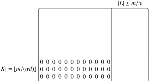
Let K ⊆ {1,2, . . . ,m}be the set of rows ofA containingbm/(αd)crows with the smallest number of non-zero entries, whereα > 2 is a constant to be determined later. By the commutativity of R, we may assume that K contains the bottommost|K|rows. LetL ={1 ≤ j ≤ n : ∃_i_∈_K : ai,j , 0}. Observe that|L| ≤ m/α, as the average

number of non-zero entries in the rows of K is at most d. Again by using the commutativity ofR, assume that L={n− |L|+1,n− |L|+2, . . . ,n}, that is, we order the columns ofAsuch that the columns ofLappear at the right of the matrix. In particular for any 1≤i≤n−m/αand j∈Kwe haveai,j=0 (see Figure 1).

Consider the following standard dynamic programming approach. For a subsetXof rows ofAand integer|X| ≤r≤ ndefinet[X,r] as the permanent of (ai,j)i∈X,1≤j≤r, a|X|×rsubmatrix ofA. Note that we are to computet[{1,2, . . . ,m},n].

Observe that the following recursive formula allows to compute the entries of the tablet, where we sum over the element used in the permanent computation in ther-th column ofA:

t[X,r]=t[X,r−1]+X

i∈X

ai,rt[X\ {i},r−1],

with the boundary conditionst[∅,r]=1 for any 0≤r≤nandt[X,r]=0 for anyr<|X|. Moreover, for computing t[{1,2, . . . ,m},n] we do not need to compute the valuest[X,r] wheren−r<m− |X|.

Let us upper bound the number of pairs (X,r) for whichn−r≥m− |X|andt[X,r] is non-zero. We consider two cases, depending onr.

First, consider the caser≤n−m/α. Recall thatai,j =0 for anyi∈ Kand j ≤n−m/α. Hence, ift[X,r],0,

thenX∩K =∅. Since|K|=bm/(αd)c, there are at mostn2m−bm/(αd)c_≤_n21+(1−1/(αd))m_{pairs (X}_,_{r) with}_t[X_,_r]

,0 and

(5)

0 0 0

0 0 0 |K|=bm/(αd)c

[image:5.595.179.423.113.245.2]

|L| ≤m/α

Figure 1: A block of zero entries in the binary matrix.

Second, consider the caser > n−m/α. Recall that we are only interested in the valuest[X,r] for pairs (X,r) satisfying n−r ≥ m− |X|. In our case this implies |X| > m(1 −1/α) and, consequently, as α > 2, there are onlym_b_mm_/α_c choices for the set X. By using the binary entropy function, we get _b_mm_/α_c = O?(2H(1/α)m_{), where}

H(p)=−plog₂p−(1−p) log₂(1−p). Ford≥2 andα=3.55 we have 2H(1/α)_≤₂1−1/(αd)_.

Consequently, to obtain the claimed running time of Theorem 1 it suffices to skip the computation of valuest[X,r] whenevern−r<m− |X|, orr≤n−m/αandX∩K,∅. This finishes the proof of Theorem 1.

We remark here that the constantα=3.55 can be improved if we have a stronger lower bound ond. However, in our analysis it is crucial thatα > 2, so that the number of subsetsX ⊆ {1,2, . . . ,m}of size|X| > m(1−1/α) is exponentially smaller than 2m_.

We would like also to observe that the assumption of commutativity ofR is essential to perform the dynamic programming algorithm in the appropriate order of rows and columns (which, in the above proof, is disguised in the operation of reordering rows and columns ofA). On the other hand, we do not need the additive inverse inR, hence the algorithm works for semirings, as claimed.

3. Counting perfect matchings in general graphs

In this section we study the problem of counting the number of perfect matchings in general graphs. We show an inclusion-exclusion based algorithm, which given ann-vertex graph computes the number of its perfect matchings in O?(2n/2) time and polynomial space. This matches the time and space bounds of the algorithm of Bj¨orklund [5].

Theorem 4. Given an n-vertex graph G=(V,E)inO?(2n/2)time and polynomial space one can count the number of perfect matchings in G.

Proof. Clearly we can assume thatnis even. Consider the edges ofGbeing black and letV ={v0, . . . ,vn−1}. Now

we add to the graph a perfect matching of red edgesER ={v2iv2i+1: 0≤i<n/2}obtaining a multigraphG0. Denote

ei=v2iv2i+1∈ER.

We say that a cycle or a walk inG0_is_{alternating, if, when we traverse the cycle (walk), the colours of the edges}

alternate; in particular, an alternating cycle or closed walk is of even length. Observe that for any perfect matching M⊆Ethe multisetM∪ERis a cycle cover (potentially with 2-cycles), where all the cycles arealternating. Moreover,

for any cycle coverYofG0_{composed of alternating cycles the set}_Y_\_E

Ris a perfect matching inG. This leads us to

the following observation.

Claim 5. The number of perfect matchings in G equals the number of cycle covers in G0where each cycle is alternat-ing.

(6)

one, but also has a designated starting point. However, note that the definition ofalternatingapplies well to (closed) walks.

We are going to compute the number of cycle covers ofG0_{with alternating cycles using the inclusion-exclusion}

principle over the set of red edgesER.

For an edgeei∈ ER, we say that a closed walkCisei-niceif it is alternating, starts withv2i,ei,v2i+1, traversesei

exactly once, and does not traverse any edgeej ∈ERfor j <i. Note that for an alternating walkC, ifCcontains a

vertexv2jorv2j₊1, it needs to traverse the edgeej∈ER, as this is the only red edge incident tov2jandv2j₊1. A closed

walk isniceif it isei-nice for someei ∈ ER; note that, in this case, the edgeei is defined uniquely. Moreover, note

that for any alternating cycleCthere is exactly one way to define a nice closed walk with the same length and set of edges asC: one needs to start with the edgeeitraversed byCof lowest possible index, and traverse it in the direction

fromv2itov2i+1.

For a positive integerrlet us define the universeΩras the set ofr-tuples, where each of thercoordinates contains

a nice closed walk inG0and the total length of all the walks equalsn. For 0 ≤ i <n/2 letAr,i ⊆ Ωr be the set of

r-tuples where at least one walk contains the arcei. We now claim the following.

Claim 6. The number of perfect matchings in G equalsP

1≤r≤n/2|T0≤i<n/2Ar,i|/r!.

Proof. By Claim 5, it suffices to focus on cycle covers ofG0where each cycle is alternating.

Consider first such a cycle coverY. In the multigraph (V,Y) each connected component is an alternating cycle. Letrbe the number of these cycles. Moreover, for each such cycleC, letW(C) be the unique nice closed walk with the same length and edge set asC. Letτ=(W1,W2, . . . ,Wr) be any ordering of the walksW(C), whereCiterates over

the set of cycles ofY. Observe thatτ ∈Ω_r, as each walkWjis nice. As each cycle ofYis alternating,ER ⊆Y and,

consequently, for any 0≤i<n/2 we haveτ∈Ar,i. Thus, each cycle coverYgives rise tor! elements ofT0≤i<n/2Ar,i

that differ on the choice of the order of walksWjin the tupleτ. Furthermore, observe that the walksWjare pairwise

disjoint (and, hence, all theser! tuples are pairwise different) and, moreover, different cycle coversY yield different tuplesτ, as their differ on the set of used edges.

In the other direction, consider a tupleτ =(W1,W2, . . . ,Wr) ∈T0≤i<n/2Ar,i. By the definition ofAr,i, each edge

ofERneeds to be contained in at least one of the walksWj. On the other hand, the total length of the walksWjisn,

while|ER|=n/2. Since the walksWjare alternating, we infer that each edgeERis traversed exactly once by exactly

one walkWj. Since each vertex ofG0is incident to exactly one edge ofER, we have that eachWjinduces a cycle in

G0, and these cycles are pairwise vertex disjoint. Hence, the set of all edges of all walks inτis a cycle cover inG0

with each cycle being alternating. The claim follows. _y

By Claim 6, it suffices to compute|T

0≤i<n/2Ar,i|for all 1≤r≤n/2. Let us now focus on a single value ofr. By

the inclusion-exclusion principle

\

0≤i<n/2

Ar,i

= X

I⊆{0,...,n/2−1}

(−1)|I|

\

i∈I

(Ωr\Ar,i)

,

where we define T

i∈I(Ωr \Ar,i) for I = ∅ asΩr. Hence to prove the theorem it is enough to compute the value

|T

i∈I(Ωr\Ar,i)|for a given 1 ≤r ≤ n/2 andI ⊆ {0, . . . ,n/2−1}in polynomial time. This is done by a standard

dynamic programing approach in the remainder of this proof.

LetG0_Ibe the graphG0with all the endpoints of edgeseifori∈Iremoved. For every 0≤a<n/2 and every even

2≤q≤n, letpa,qbe the number ofea-nice closed walks inG0I of lengthq. We first show how to compute each value

pa,qin polynomial time.

To this end, for every 2a+1≤i<nand every odd 0<qˆ<qdefinetp[i,q] as the number of alternating walksˆ W

of length ˆqinG0_I, where each walk starts withv2a,ea,v2a+1, ends withvi⊕2,ebi/2c,vi, visitseaonly once and does not

visit any edgeecforc<a. It is straightforward to verify thattp[i,q] satisfies the following boundary conditions:ˆ

tp[2a+1,1]=1

tp[i,1]=0 fori,2a+1

(7)

and the following recurence relation for every 2a+1<i<nand every odd 3≤qˆ<q:

tp[i,q]ˆ =

X

vi⊕1vj∈E(G0I)

2a+1≤j<n

tp[j,qˆ−2].

Hence, the valuestp[i,q] can be computed in polynomial time. Finally, observe thatˆ

pa,q=

X

vavi∈E(G0I)

2a+1≤i<n

tp[i,q−1].

Having the values pa,q, we now show how to compute|Ti∈I(Ωr \Ar,i)|by the standard knapsack type dynamic

programming. That is, for every 0≤rˆ≤rand every even 0 ≤q ≤nwe definet[ˆr,q] to be the number of ˆr-tuples of nice closed walks inG0_I of total lengthq. It is straightforward to verify thatt[ˆr,q] satisfies the following boundary conditions:

t[0,0]=1

t[ˆr,0]=t[0,q]=0 for ˆr,q>0

and the following recurence relation for every 0<ˆr≤rand every even 0<q≤n:

t[ˆr,q]= X

0<qˆ<q ˆ qeven

t[ˆr−1,q]ˆ X

0≤a<n/2 a_<I

pa,q−qˆ.

Hence, the valuest[ˆr,q] can be computed in polynomial time. Finally, observe that

\

i∈I

(Ωr\Ar,i)

=t[r,n].

This concludes the proof of Theorem 4.

4. Properties of bounded average degree graphs

This section contains technical results concerning bounded average degree graphs. In particular we prove Lemma 12, which bounds the number of “Hamiltonian-like” structures in a graph and is needed to get the claimed running times in Theorems 2 and 3. However, as the proofs of this section are not needed to understand the algorithms in Section 5 the reader may decide to see only Definition 11 and the statement of Lemma 12.

We start with a few well-known bounds.

Lemma 7. For any n≥k≥1it holds that

n k !

≤ _en

k k

.

Moreover, the upper bounding function x7→(en/x)x_{is nondecreasing on the domain}₀_<_x_≤_n.

Proof. For the first claim, observe that

n k !

≤n

k

k! ≤n

ke

k k

,

where the last inequality follows from the Stirling’s approximation of the factorial function. For the second claim, substitutey=n/xand observe thaty7→y−1_ln_y_{is nonincreasing for}_y_≥_1.

(8)

Proof. It is well-known that limn→∞Hn−lnn=γwhereγ >0.577 is the Euler-Mascheroni constant and the sequence

Hn−lnnis decreasing. ThereforeHn−1 =Hn−1_n ≥lnn+γ−1_n, hence the lemma is proven forn≥2 asγ > 1₂. For

n=1, note thatHn−1=lnn=0.

The following lemma helps us identify disjoint parts of the input graph where we can independently save on the number of “Hamiltonian-like” structures, provided that we have already bound the maximum degree of the graph.

Lemma 9. Given an n-vertex graph G=(V,E)of average degree at most d and maximum degree at most D one can in polynomial time find a set A containingd₂₊_4dDn evertices of degree at most2d, where for each x,y∈A, x ,y we

have NG[x]∩NG[y]=∅.

Proof. Note that|Vdeg≤2d| ≥n/2. We apply the following procedure. Initially we setA:=∅and all the vertices are

unmarked. Next, as long as there exists an unmarked vertex xinVdeg≤2d, we add xtoA and mark all the vertices

NG[NG[x]]. Since the setNG[NG[x]] contains at most 1+2d+2d(D−1)=1+2dDvertices, at the end of the process

we have|A| ≥ n

2+4dD. Clearly this routine can be implemented in polynomial time.

The next lemma states that, although in ann-vertex graph of average degree at mostdthere may be up tond

D vertices

of degree at leastD, this bound cannot be tight for a large range of values ofDat once. This simple observation is in fact the main source of the gain in bounds proven in Lemma 12.

Lemma 10. For anyα≥0and an n-vertex graph G =(V,E)of average degree at most d there exists D≤eαsuch that|Vdeg>D| ≤ _αnd_D.

Proof. By standard counting arguments we have

∞

X

i=0

|Vdeg>i|=

∞

X

i=0

i|Vdeg=i| ≤nd.

For the sake of contradiction assume that|Vdeg>i|> nd_αi, for eachi≤e

α_{. Then}

∞

X

i₌0

|Vdeg>i| ≥

beαc

X

i₌1

|Vdeg>i|>

nd

α

beαc

X

i₌1

1/i= nd

αHbeαc≥nd,

where the last inequality follows from Lemma 8.

In the following definition we capture “Hamiltonian-like” structures in a graph. The family of all these struc-tures contains the family of the sets used in the dynamic programming algorithms for TSP-like problems (that is, in Theorems 2 and 3).

Definition 11. For an undirected multigraph G =(V,E)and two vertices s,t ∈ V bydeg2sets(G,s,t)we define the set of all subsets X⊆V\ {s,t}, for which there exists a set of edges F ⊆E such that:

• deg_F(v)=0for each v∈V\(X∪ {s,t}),

• deg_F(v)=2for each v∈X,

• deg_F(v)≤1for v∈ {s,t}.

We are now ready to state and prove the main result of this section.

Lemma 12. For every d≥1there exists a constantεd >0, such that for an n-vertex multigraph G =(V,E)without

(9)

Proof. We begin with invoking Lemma 10 to get a partition of V into high- and low-degree vertices. Let cbe a sufficiently large universal constant; it suffices to takec =20. Lemma 10, invoked onGandα :=ecd, provides us with an integerD ≤eα =eecd

such that there are at most nd

αD vertices of degree greater thanDinG. Recall that the

standard averaging argument provides us with only and_D upper bound on|Vdeg>D|; we are going to heavily rely on the

fact that|Vdeg>D|is in factαtimes smaller than this bound.

The thresholdDprovided by Lemma 10 may turn out to be even smaller thandso, for technical reasons, we are going to use a slightly adjusted thresholdD0:=max(2d,D). Observe thatD0 ≤eαasd ≥1 implies 2d ≤eαfor any c≥1. LetH=G[Vdeg≤D0] be the subgraph induced by the low-degree vertices and letY =V_deg_>_D0be the (remaining)

set of high-degree ones. Note that the bound of Lemma 10 implies that|Y| ≤_αnd_D, asD0≥DandY ⊆Vdeg>D.

The main reason why we have adjusted the threshold fromDtoD0is thatD0≥2dimplies thatHcontains at least n/2 vertices. Moreover, asHcontains all low-degree vertices ofG, the average degree ofHis not greater than the average degree ofG, which in turn is bounded byd.

AsH has boundedmaximumdegree byD0, we may apply Lemma 9 to get a large family of pairwise disjoint closed neighbourhoods inH. Formally, we can in polynomial time construct A⊆V(H) ofdn/(4+8dD0₎_e_vertices,

each of degree at most 2d, and withNH[v]∩NH[w]=∅for anyv,w∈A,v,w.

Let us now give an informal overview of the purpose of the setA. Assume for a moment thatY=∅, that is, there are no high-degree vertices andG = H. Consider a setX ∈ deg2sets(G,s,t) and a corresponding setF ⊆E from Definition 11. The crucial observation is that for anyv∈A\ {s,t}, the setX∩N[v] cannot be equal to{v}, asvneeds to be of degree 2 inFandGdoes not contain any self-loops by the assumptions of the lemma. Consequently, out of 2|N[v]|_{choices for}_X_∩_{N[v], at least one is invalid, and}

deg2sets(G,s,t) ≤2

n_·Y

v∈A

2|N[v]|−1 2|N[v]| ≤2

n_· ₁₋ 1

22d+1

!|A|

. (1)

If|A|isΩ(n), such a statement would finish the proof of the lemma. However, in the general caseYmay not be empty, andX∩NH[v]={v}for somev∈A\ {s,t}if both edges ofFincident tovhave their second endpoints inY. Luckily,

|Y|is very small thanks to Lemma 10 and may “disturb” the argument of (1) only for a small part ofA. Thus, to count setsX∈deg2sets(G,s,t), for each choice of small subset ofAthat get “disturbed” by the elements ofY, we apply the argument of (1) to the remainder ofA. Thanks to the bound on|Y|, the gain from the argument of (1) is larger than the overhead we get from enumerating all sets of vertices ofA“disturbed” byY.

Let us now proceed with a formal argumentation. First, we rephrase the bound on|A|so that it is more convienient in the future. Sinced≥1 andD0≥2d, we have:

|A|= _n

4+8dD0

≥ n

4+8dD0 ≥

n

2dD0₊_8dD0 =

n

10dD0. (2)

Ifn≤ 8edD₄₋_e0,n=O(1) and the claim of the lemma is trivial. Otherwise:

|A|= _n

4+8dD0

< n

8dD0+1<

n

2edD0. (3)

Recall that, by Lemma 10,|Y|is very small, namely|Y| ≤ _αnd_D. We now formally show that|Y|is much smaller than|A|. Asd≥1 andD0=max(2d,D)≤2dD, for sufficiently largecwe have:

|Y| ≤ nd

αD ≤ n 20dD0 ·

40d3

ecd ≤

|A| 2 ·

40d3

ecd <

|A|

2 . (4)

For an arbitrary setX ∈deg2sets(G,s,t), and a corresponding setF ⊆Efrom Definition 11, defineZX as the set

of verticesx∈(X∩V(H))\ {s,t}such thatNH(x)∩X=∅. Intuitively, these are the vertices that get “disturbed” byY

in the argument of (1). Formally, recall thatFis a set of paths and cycles, where each vertex ofZX is of degree two.

HenceFcontains at least 2|ZX|edges betweenZX andY, as any path/cycle ofF visiting a vertex ofZX has to enter

(10)

By the definition ofZX, for eachx∈A\(ZX∪ {s,t}) we have thatNH[x]∩X,{x}and|NH[x]| ≤2d+1. Recall

that ifx∈A∩ZX, we haveNH[x]∩X={x}. Therefore, following the lines of (1), we have that for fixedA∩ZXthere

are at most

2n 2

2d+1₋₁

22d+1

!|A\(ZX∪{s,t})|

1 2

!|A∩ZX|

≤2n+2 2

2d+1₋₁

22d+1

!|A|

(5)

choices forX∈deg2sets(G,s).

As|ZX| ≤ |Y|and|Y|is much smaller than|A|, we can bound the number of choices ofA∩ZXin a straightforward

manner: there are at mostP|Y|

i=0

_|_A_|

i

≤n|_|A_Y|_|choices forA∩ZX. Thus

|deg2sets(G,s,t)| ≤2n+2· 2

2d+1₋₁

22d₊1

!|A| ·n |A|

|Y| !

. (6)

It remains to estimate|_|A_Y|_|. To this end, we use Lemma 7 as follows:

|A| |Y| !

≤ e|A| |Y|

!|Y|

by Lemma 7

≤ e· n 2edD0·

1 |Y|

!|Y|

by (3)

≤

e· n 2edD0 ·

αD nd

αndD

by|Y| ≤ nd

αD≤ n

2edD0 (cf.(4)) and by Lemma 7

≤ α

2d2

_αnd_D

sinceD≤D0

< αnd

αD. ₍₇₎

We now proceed to the final calculations, putting all obtained bounds together. By the standard inequality 1−x≤ e−xwe have that

(22d+1−1)/22d+1 =(1−1/22d+1)≤e−1/22d+1. (8)

Using (2), (7) and (8) we obtain that

|A|

|Y| !

22d+1−1 22d+1

!|A|/2

≤exp ndlnα

αD − n 20dD0₂2d+1

!

.

Plugging inα=ecdand using the fact thate10d >40d3ford≥1 we obtain:

|A| |Y|

!

22d+1₋₁

22d₊1

!|A|/2

≤exp ncd

e(c−10)d_20d_·_2dD −

n 20dD0₂2d₊1

!

.

SinceD0=max(2d,D)≤2dDande5d>d22d+1_as_d_≥_{1, we get}

|A| |Y|

!

22d+1−1 22d+1

!|A|/2 ≤exp

_n

20dD0₂2d+1

_c

e(c−15)d −1

.

Finally, for sufficiently largec, asd≥1, we havec<e(c−15)d_and

|A|

|Y|

! ₂2d+1₋₁

22d+1

!|A|/2

(11)

Consequently, we obtain:

|deg2sets(G,s,t)| ≤2n+2· 2

2d+1₋₁

22d+1

!|A| ·n |A|

|Y| !

by (6)

=n2n+2·       

|A|

|Y|

! ₂2d+1₋₁

22d+1

!|A|/2      

· 2

2d+1₋₁

22d+1

!|A|/2

<n2n+2 2

2d+1₋₁

22d+1

!|A|/2

by (9)

≤n2n+2exp − 1 22d₊1 ·

|A| 2

!

by (8)

≤n2n+2exp

− n

22d+1_·_20dD0

by (2)

≤n2n+2exp

− n

22d+1_·_20d_·_eecd

asD0≤eα.

This concludes the proof of the lemma. Note that the dependency ondin the final constantεd is doubly-exponential.

5. Trimming dynamic programming algorithms in graphs of bounded average degree

5.1. Minimum weight Hamiltonian cycle

To prove Theorem 2, it suffices to solve inO?(2(1−εd)n_{) time the following problem. We are given an undirected}

n-vertex graphG=(V,E) of average degree at mostd, verticesa,b ∈Vand a cost functionc:E →_R+. We are to find the cheapest Hamiltonian path betweenaandbinG, or verify that no Hamiltonianab-path exists.

We solve the problem by the standard dynamic programing approach. That is for eacha ∈X ⊆V andv∈ Xwe computet[X,v], which is the cost of the cheapest path fromatovwith the vertex setX. The entryt[V,b] is the answer to our problem. Note that it is enough to consider only such pairs (X,v), for which there exists anav-path with the vertex setX.

We first sett[{a},a] = 0. Then iteratively, for eachi = 1,2, . . . ,n−1, for eachu ∈ V, for each X ⊆ V such that |X| = i, a,u ∈ X andt[X,u] is defined, for each edgeuv ∈ E wherev < X, ift[X ∪ {v},v] is undefined or

t[X∪ {v},v]>t[X,u]+c(uv), we sett[X∪ {v},v]=t[X,u]+c(uv).

Finally, note that ift[X,v] is defined then X \ {a,v} ∈ deg2sets(G,a,v). Hence, the complexity of the above algorithm is within a polynomial factor fromP

v∈V|deg2sets(G,a,v)|, which is bounded byO?(2(1−εd)n) by Lemma 12.

5.2. Counting perfect matchings

In this section we show how the algorithm from Section 3 can be reformulated as a dynamic programming routine (using exponential space), which together with Lemma 12 will imply the running time claimed in Theorem 3. Note that this reformulation causes the space complexity to be exponential.

Assume that we are given ann-vertex undirected graphG = (V,E), wheren is even, and we are to count the number of perfect matchings inG. We start with a small technical detour to ensure that the complement ofGhas perfect matching; the motivation for this step will become clear later.

Lemma 13. Given an n-vertex graph G=(V,E)with average degree at most d, one can in polynomial time identify a set X of at most4d+4vertices of G such that the complement of G\X contains a perfect matching.

Proof. Ifn≤4d+4, we may outputX :=V, so assume othewise. Construct a setY ⊆V as follows: initiateY =∅ and, as long as|Y|<2dand there exists a vertexv∈V\Ywith|N(v)\Y|>|V\Y|

2 −1, addvtoY.

(12)

As the construction of Y stopped by triggering the second condition, the complement ofG\Y has minimum degree at least|V\Y|/2 and, by Dirac’s theorem, it contains a Hamiltonian cycle. DefineX=Y if|V\Y|is even and X=Y∪ {v}, wherevis an arbitrary vertex ofV\Y, if|V\Y|is odd. In this manner|X|<2d+1 and the complement ofG\X contains a Hamiltonian path and has even number of vertices. Note that selecting every other edge of a Hamiltonian path gives us a perfect matching inG\X. This concludes the proof of the lemma.

We preprocess the input graphG = (V,E) as follows. We compute the setX using Lemma 13 and add |X|/2 connected components isomorphic to K2 to the graphG. In this manner, the complement ofG contains a perfect

matching: the new vertices can be matched to the vertices ofX and the complement of G\X contains a perfect matching by Lemma 13. Moreover, note that the number of perfect matchings ofGdoes not change, the number of vertices ofGincreases only by an additive factor of at most 4d+4, which is a constant, and the new graph has still average degree bounded byd(recalld≥1).

Thus, by using the aforementioned preprocessing, we may henceforth focus only on the case when the complement of the inputn-vertex graphG=(V,E) contains a perfect matching. Order the vertices ofGasv0,v1, . . . ,vn−1, so that

v2iv2i+1<Efor any 0≤i<n/2.

We are going to construct an undirected multigraphG0_{having only}_n_/_{2 vertices, where the edges of}_G0_{will be}

labeled with unordered pairs of vertices ofG, that is, with edges ofG. As the set of vertices ofG0₌_(V0_,_E0_{) we take}

V0₌_{_v0

0, . . . ,v

0

n/2−1}. For each edgevavbofGwe add toG

0_{exactly one edge:}_v0 ba/2cv

0

bb/2clabeled with{va,vb}. For an

edgee0_∈_E0_by_`_(e0_{) let us denote the label of}_e0_{. Note that}_G0_{may contain parallel edges but, due to the preprocessing}

step,G0_{does not contain self-loops. In other words, the preprocessing step allows us to use Lemma 12 on the graph}

G0.

Observe also that if the graphGis of average degree at mostd, then the graphG0is of average degree at most 2d. In what follows we count the number of particular cycle covers ofG0, where we use the labels of edges to make sure that a cycle going through a vertexv0_i ∈V0never uses two edges ofG0corresponding to two edges ofGincident to the same vertex.

Lemma 14. The number of perfect matchings in G equals the number of cycle covers C⊆E0of G0, whereS

e∈C`(e)=

V.

Proof. We show a bijection between perfect matchings in G and cycle covers C of G0 _{satisfying the condition}

S

e∈C`(e)=V.

LetMbe a perfect matching inG. As f(M) we definef(M)={v0 ba/2cv

0

bb/2c:vavb∈ M}. Note that f(M) is a cycle

cover and moreoverS

e∈f(M)`(e)=V. In the reverse direction, for a cycle coverC⊆E0ofG0, consider a set of edges

h(C) defined ash(C)={`(e) : e∈C}. Clearly the conditionS

e∈C`(e)=Vimplies thath(C) is a perfect matching,

and moreoverh= f−1_.

Observe, that if a cycle coverC⊆E0ofG0does not satisfyS

e∈C`(e)=V, then there is a vertexv0i ∈V

0_{, such that}

the two edges ofCincident tov0_ido not have disjoint labels. Intuitively this means we are able to verify the condition S

e∈C`(e)=Vlocally, which is enough to derive the following dynamic programming routine. Lemma 15. In O?(P

s,t∈V|deg2sets(G0,s,t)|)time and space, one can compute the number of cycle covers C of G0

satisfyingS

e∈C`(e)=V.

Proof. Anordered r-cycle coverof a graphHis a tuple ofrcycles inH, whose union is a cycle cover ofH. As each cycle cover ofHthat contains exactlyrcycles can be ordered into exactlyr! different orderedr-cycle covers, it is sufficient to count, for any 1≤r≤n/2, the number of orderedr-cycle coversCinG0_{such that each two edges in}_C

have disjoint labels. In the rest of the proof, we focus on one fixed value ofr.

For 0≤q≤randX⊆V0_as_t[q_,_{X] let us define the number of ordered}_{q-cycle covers in}_G0_{[X] where each two}

edges have disjoint labels; note thatt[r,V0] is exactly the value we need. Moreover for 0≤q<r,X⊆V0,v0_a,v0_b∈X, a<bandζ∈ {2b,2b+1}ast2[q,X,v0a,v

0

b, ζ] we define the number of pairs (C,P) where all the following conditions

hold:

• Cis an orderedq-cycle cover ofG0[Y] for someY ⊆X\ {v0a,v0b};

• Pis av0

av0b-path with the vertex setX\Ythat does not contain any vertexv

0

(13)

• any two edges ofC∪Phave disjoint labels;

• the label of the edge ofPincident tov0acontainsv2a; and

• the label of the edge ofPincident tov0

bcontainsvζ.

Note that we have the following border values:t[0,∅]=1 andt[0,X]=0 forX,∅.

Consider an entryt2[q,X,v0a,v0b, ζ], and let (C,P) be one of the pairs counted in it. We have two cases: eitherPis

of length 1 or longer. The number of pairs (C,P) in the first case equals

t[q,X\ {v0_a,v_b0}]· |{v0_av0_b∈E0:`(v0_av0_b)={v2a,vζ}}|.

In the second case, letv0_cv0_bbe the last edge ofP; note thatc>aby the assumptions onP. The label ofv0_cv0_bequals {v2c,vζ}or{v2c+1,vζ}. Thus, the number of elements (C,P) in the second case equals

X

v0_c∈X\{v0_a,v0_b}

a<c

X

η∈{2c,2c+1}

t2[q,X\ {v0b},v

0

a,v

0

c, η⊕1]· |{v

0

cv

0

b∈E

0_:_`_(v0

cv

0

b)={vη,vζ}}|.

Let us now move to the entryt[q,X] and letCbe an orderedq-cycle cover inG0_{[X]. Let}_W _{be the last cycle of}

C. Observe that, sinceG0_{does not contain any self-loops,}_W_{is of length at least two. Let}_v0

abe the lowest-numbered

vertex onW and lete = v0

av0b be the edge ofW wherev2a+1 ∈ `(e). Note that bothv

0

a andeare defined uniquely;

moreover,a<band no vertexv0_cwithc<abelongs toW. Thus

t[q,X]= X

v0a,v0_b∈X a<b

X

ζ∈{2b,2b+1}

t2[q−1,X,v0a,v

0

b, ζ⊕1]· |{v

0

av

0

b∈E

0_:_`_(v0

av

0

b)={v2a+1,vζ}}|.

So far we have given recursive formulas, that allow computing the entries of the tablestandt2. However the values

t[q,X],t2[q,X,v0a,v

0

b, ζ] forX <

S

s,t∈V0deg2sets(G0,s,t) are equal to zero. The last step of the proof is to show how

to perform the dynamic programming computation in a time complexity within a polynomial factor from the number of non-zero entries of the table. We do that in a bottom-up manner, that is iteratively, for eachq =0,1,2, . . . ,r, for eachi=1,2, . . . ,n, we want to compute the values of non-zero entriest[q,X] for all setsXof cardinalityiand then compute the values of non-zero entriest2[q,X,∗,∗,∗] for all setsXof cardinalityi.

Whenever we compute some valuet[q,X] ort2[q,X,∗,∗,∗] and it turns out to be non-zero, we enqueue for further

computation all valuest[q0_,_X0_{] or}_t

2[q0,X0,∗,∗,∗] for which the currently computed value contributes to in the

recur-sive formulae. Observe that each valuet[q,X] oft2[q,X,∗,∗,∗] contributes to a polynomial number of applications

of the recursive formulae. We process the valuest[q,X] andt2[q,X,∗,∗,∗] in the aforementioned order (i.e., in the

increasing order ofqand|X|, and, for fixedqandX, firstt[q,X] and thent2[q,X,∗,∗,∗]), but we only focus on the

cells that were previously enqueued.

The single non-zero value that we start with ist[0,∅]= 1. (Note thatt[0,X] =0 forX ,∅.) This finishes the

proof of the lemma.

Theorem 3 follows directly from the Lemma 12 together with Lemma 15.

6. Conclusions

In our work we have shown how the assumption of bounded average degree of a graph can provide exponential speed up in the classic dynamic programming routines. Very recently Golovnev et al. [20] proved that the dynamic programming algorithms of Theorems 2 and 3 can be turned into polynomial-space algorithms by using algebraic techniques. Moreover, they also showed how to use the gap obtained in Lemma 10 to compute the chromatic number of a graph of average degreedwith exponential speedup over theO?(2n_{)-time algorithm [21]. We believe our approach,}

(14)

Acknowledgements

We would like to thank anonymous referees for their helpful remarks and comments.

This research has been partially supported by NCN grant N206567140 and Foundation for Polish Science.

[1] R. Bellman, Dynamic programming treatment of the travelling salesman problem, J. ACM 9 (1962) 61–63.

[2] M. Held, R. M. Karp, A dynamic programming approach to sequencing problems, J. Soc. Ind. Appl. Math. 10 (1962) 196–210.

[3] G. J. Woeginger, Exact algorithms for NP-hard problems: A survey, in: M. J¨unger, G. Reinelt, G. Rinaldi (Eds.), Combinatorial Optimization, Vol. 2570 of Lecture Notes in Computer Science, Springer, 2001, pp. 185–208.

[4] H. Ryser, Combinatorial Mathematics, The Carus Mathematical Monographs, Mathematical Association of America, 1963. [5] A. Bj¨orklund, Counting perfect matchings as fast as Ryser, in: Y. Rabani (Ed.), SODA, SIAM, 2012, pp. 914–921. [6] A. Bj¨orklund, Determinant sums for undirected hamiltonicity, in: FOCS, IEEE Computer Society, 2010, pp. 173–182.

[7] R. Impagliazzo, R. Paturi, On the complexity ofk-SAT, J. Comput. Syst. Sci. 62 (2) (2001) 367–375.

[8] M. Cygan, H. Dell, D. Lokshtanov, D. Marx, J. Nederlof, Y. Okamoto, R. Paturi, S. Saurabh, M. Wahlstr¨om, On problems as hard as CNF-SAT, in: IEEE Conference on Computational Complexity, IEEE Computer Society, 2012, pp. 74–84.

[9] D. Lokshtanov, D. Marx, S. Saurabh, Known algorithms on graphs on bounded treewidth are probably optimal, in: D. Randall (Ed.), SODA, SIAM, 2011, pp. 777–789.

[10] M. Pˇatras¸cu, R. Williams, On the possibility of faster SAT algorithms, in: M. Charikar (Ed.), SODA, SIAM, 2010, pp. 1065–1075.

[11] E. T. Bax, J. Franklin, A permanent algorithm with exp(Ω(n13)/2 lnn) expected speedup for 0-1 matrices, Algorithmica 32 (1) (2002) 157–

162.

[12] R. A. Servedio, A. Wan, Computing sparse permanents faster, Inf. Process. Lett. 96 (3) (2005) 89–92.

[13] T. Izumi, T. Wadayama, A new direction for counting perfect matchings, in: FOCS, IEEE Computer Society, 2012, pp. 591–598.

[14] A. Bj¨orklund, T. Husfeldt, P. Kaski, M. Koivisto, Evaluation of permanents in rings and semirings, Inf. Process. Lett. 110 (20) (2010) 867–870.

[15] A. Bj¨orklund, T. Husfeldt, Exact algorithms for exact satisfiability and number of perfect matchings, Algorithmica 52 (2) (2008) 226–249. [16] M. Koivisto, Partitioning into sets of bounded cardinality, in: J. Chen, F. V. Fomin (Eds.), IWPEC, Vol. 5917 of Lecture Notes in Computer

Science, Springer, 2009, pp. 258–263.

[17] A. Bj¨orklund, T. Husfeldt, P. Kaski, M. Koivisto, The traveling salesman problem in bounded degree graphs, ACM Transactions on Algo-rithms 8 (2) (2012) 18.

[18] A. Bj¨orklund, T. Husfeldt, P. Kaski, M. Koivisto, Fourier meets M¨obius: fast subset convolution, in: D. S. Johnson, U. Feige (Eds.), STOC, ACM, 2007, pp. 67–74.

[19] A. Bj¨orklund, T. Husfeldt, P. Kaski, M. Koivisto, Trimmed M¨obius inversion and graphs of bounded degree, Theory Comput. Syst. 47 (3) (2010) 637–654.

[20] A. Golovnev, A. S. Kulikov, I. Mihajlin, Families with infants: a general approach to solve hard partition problems, CoRR abs/1311.2456.