1 ECE-320: Linear Control Systems
Homework 2
Due: Monday March 21, 2016 at the beginning of class
1) An ideal second order system has the transfer function
G s
o( )
. The system specifications for a step input are asfollows:
Percent Overshoot < 5%, Settling Time < 4 seconds (2% criteria), Peak Time < 1 second
Sketch, in the complex plane, the permissible area for the poles of
G s
o( )
in order to achieve the desired response.2) For systems with the following transfer functions:
1 6
( ) ( )
2 ( 2)( 3)
a b
H s H s s
s s s
a) Determine the unit step and unit ramp response for each system using Laplace transforms. Your answer should be time domain functions ya (t) and yb (t) .
b) From these time domain functions, determine the steady state errors for a unit step and unit ramp input.
The following Matlab code can be used to estimate the step and ramp response for 5 seconds for transfer function Hb (s)
H = tf([1 6],[1 5 6]); % enter the transfer function
t = [0:0.01:5]; % t goes from 0 to 5 by increments of 0.01 ustep = ones(1,length(t)); % the step input is all ones, u(t) = 1; uramp = t; % the ramp input is has the input u(t) = t; ystep = lsim(H,ustep,t); % find the step response
yramp = lsim(H,uramp,t); % find the ramp response
figure; % make a new figure
orient tall % or orient landscape, use more of the page subplot(2,1,1); % put two graphs on one piece of paper plot(t,ustep,'.-',t,ystep,'-'); % plot input/output with different line types
grid; % put a grid on the graph
legend('Step Input','Step Response',4); % put a legend on the graph
subplot(2,1,2); % second of two graphs on one piece of paper plot(t,uramp,'.-',t,yramp,'-'); % plot input/output with different line types
grid; % put a grid on the graph
legend('Ramp Input','Ramp Response',4); % put a legend on the graph
c) Plot the step and ramp response for both systems (a and b) and indicate the steady state errors on the graph. Draw on the graph to show you know what the steady state errors are.
2
3) The differential equation model of an ideal second order system is
2 2
( ) 2
n( )
n( )
= K
n(
)
y t
y t
y t
x t
Here Kis the static gain,
nis the natural frequency, and is the damping ratio. These are the parameters we need to determine for these models.You will need to download and uncompress the file Homework2 Files.rar. The Matlab file
second_order_driver.m reads in data from a file (the measured data files for an unknown system) and extracts the time, input, and output values for the system. After this, you are to modify your guesses for the damping ratio, the natural frequency, and the static gain. The Matlab script second_order_driver.m then runs the Simulink model file Second_Order_System.mdl and plots the results of your model with the measured data.
You are to change the parameters in the Matlab driver file to try and get your model to match the step response of the unknown system as well as possible. Once you are done, save the graph with the step responses of the two systems and put it in your memo.
You will need to do this for the data files measured_1, measured_2, measured_3, and measured_4.
Your homework should contain four figures for this problem.
4) One of the methods that can be used to identify and
nfor mechanical systems the log-decrement method,which we will derive in this problem. If our system is at rest and we provide the mass with an initial displacement away from equilibrium, the response due to this displacement can be written
1
( )
cos(
)
nt
d
x t
Ae
t
where1
( )
x t
= displacement of the mass as a function of time = damping ratio
n
= natural frequencyd
= damped frequency = n 12After the mass is released, the mass will oscillate back and forth with period given by d 2
d
T
, so if we measure
the period of the oscillation (
T
d) we can estimate
d.Let's assumet
0is the time of one peak of the cosine. Sincethe cosine is periodic, subsequent peaks will occur at times given by
t
n
t
0nT
d, wheren
is an integer.a) Show that 1 0
1
( ) ( )
n dT n
n x t e x t
b) If we define the log decrement as 1 0 1
( ) ln
( )n x t x t
show that we can compute the damping ratio as
2 2 2
3
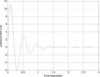
[image:3.612.126.480.91.363.2]c) Given the initial condition response shown in the Figures on the next page, estimate the damping ratio and natural frequency using the log-decrement method. (You should get answers that include the numbers 15, 0.2, 0.1 and 15, approximately.)
Figure 1. Initial condition response for second order system A.
[image:3.612.128.478.415.684.2]4
5) For the following systems
a) Determine the system type (0, 1, 2, ...)
b) If the system is type 0 assume Gpf 1and determine the position error constant Kp and the steady state error
for a unit step input. Then determine the value of Gpf to make this error zero. If the system is type 1, assume
1 pf
G and determine the steady state error for a unit step, the velocity error constant Kv, and the steady state error for a unit ramp.
Ans. (steady state errors) 3
2
, 3
13, 3 5
, 1
2; (prefilers) 2 5,
13 10
+ -
+ -
+ - +
5
6) (root locus construction) For the following problem, assume we are using the following control system
where the plant is given by
2
1 1
( )
4 29 ( 2 5 )( 2 5 )
p G s
s s s j s j
For the following controllers, sketch the root locus with arrows showing the direction of travel as k increases. If there are any poles going to zeros at infinity, you need to compute the centroid of the asymptotes (c) and the angles of the asymptotes.
You may (and should) check your answers with Matlab (use the rlocus command), but you need to do this by hand.
a) G sc( )k ( proportional (P) controller)
b) G sc( ) k s
(an integral (I) controller)
c) G sc( ) k s( z) s
(a proportional + integral (PI) controller) Write the centroid cas a function of z. For what
values of z will the two asymptotes be in the right half plane? (For plotting purposes, assume z is equal to 2.)
d) G sc( )k s( z) (a proportional+derivative (PD) controller) (For plotting purposes, assume z is equal to 2.)
e) ( ) ( 1)( 2)
c
k s z s z
G s
s
(a proportional+integral+derivative (PID) controller) Sketch this for the case where
both zeros are real and then when both zeros are complex conjugates.
f) ( ) ( )
( )
c
k s z
G s
s p
( a lead controller, pz) Write an expression for cas a function of the distance
between the pole and the zero, l p z. What happens to the asymptotes as l gets larger? (For plotting purposes, assume p is 5 and z is 1.)
6
7) (root locus construction) For the following problem, assume we are using the following control system
where the plant is given by
1 ( )
3 p
G s s
For the following controllers, sketch the root locus with arrows showing the direction of travel as k increases. If there are any poles going to zeros at infinity, you need to compute the centroid of the asymptotes (c) and the angles of the asymptotes.
You may (and should) check your answers with Matlab (use the rlocus command), but you need to do this by hand.
a) G sc( )k ( proportional (P) controller)
b) G sc( ) k s
(an integral (I) controller)
c) c( ) ( )
k s z
G s
s
(a proportional + integral (PI) controller) Sketch this for the case when z is equal to 2
and then assume z is equal to 4; there will be two plots.
d) G sc( )k s( z) (a proportional+derivative (PD) controller) Sketch this for the case where z is equal to 2 and then assume z = 4; there will be two plots.
e) ( ) ( 1)( 2)
c
k s z s z
G s
s
(a proportional+integral+derivative (PID) controller) Sketch this for the case where
there are zeros at 4 4j and when they are at -6 and -8; there will be two plots.