Discovery and Quantification of Open DNS Resolvers on IPv6

(1)

U

NIVERSITY OF

T

WENTE

M

ASTER

T

HESIS

Discovery and Quantification of Open

DNS Resolvers on IPv6

Author:

Tim KLEINNIJENHUIS Examination Committee:Prof.dr.ir. Aiko PRAS dr. Anna SPEROTTO dr. Andreas PETER Luuk HENDRIKS, MSc

A thesis submitted in fulfillment of the requirements for the degree of Master of Embedded Systems

in the

Design and Analysis of Communication Systems Group

(2)

i

University of Twente

Abstract

Faculty of Electrical Engineering, Mathematics and Computer Science

Master of Embedded Systems

Discovery and Quantification of Open DNS Resolvers on IPv6

by Tim KLEINNIJENHUIS

(3)

ii

List of Figures

1.1 Example DNS tree with a number of nodes . . . 2

1.2 Source IP address spoofing . . . 5

3.1 ASN of the verified open resolvers of the 1% subset of the IPv6 ad-dress list . . . 15

4.1 ASN of the verified open resolvers of the IPv6 address list . . . 20

4.2 The number of hitlists where the IPv6 addresses are found in . . . 21

5.1 Answer message size in bytes of the query to the open resolvers of the IPv6 address list . . . 24

5.2 Amplification factor with the frame length as message size . . . 25

5.3 Amplification factor with the IPv6 payload size as message size . . . . 26

5.4 Hamming weight of the IIDs of the open and verified resolvers rep-resented by the blue line, and the hamming weight of equally many random generated IIDs represented by the red line. . . 29

5.5 Hamming weight of the IIDs of the resolvers successfully resolving the full zone represented by the blue line, and the hamming weight of equally many random generated IIDs represented by the red line . . . 30

5.6 Hamming weight of the IIDs of the resolvers successfully resolving the small zone represented by the blue line, and the hamming weight of equally many random generated IIDs represented by the red line . . 30

5.7 Bandwidth measurement of the 100 Megabit resolver using the mea-surement machine. . . 32

5.8 Bandwidth measurement of the 100 Megabit resolver using the high speed network capturing machine . . . 33

5.9 Bandwidth measurement of the 1 Gigabit resolver using the measure-ment machine . . . 33

(6)

v

List of Tables

1.1 Common DNS queries . . . 3

1.2 Resolvers found by the Open Resolver Project . . . 4

3.1 Difference in the number of open resolvers and validated resolvers in the 1% subset of the IPv6 address list . . . 14

3.2 Open and validated resolvers of the 1% subset of the IPv6 address list, and the ratio between open and validated resolvers and the total entries in the subset . . . 15

4.1 Difference in the number of open resolvers and validated resolvers of the IPv6 address list. . . 18

4.2 Open and validated resolvers of the IPv6 address list, and the ratio between open and validated resolvers and the total entries in the ad-dress list . . . 19

4.3 The number of hitlists where the IPv6 addresses are found in . . . 20

5.1 The highest, lowest, mean and median value, in bytes, of the message size of the successful queries. . . 23

5.2 The highest, lowest, mean and median value, in bytes, of the message size of the failed queries . . . 23

5.3 The highest, lowest, mean and median value of the amplification fac-tor, with frame-len as message size . . . 26

5.4 The highest, lowest, mean and median value of the amplification fac-tor, with ipv6-plen as message size . . . 27

5.5 The highest, lowest, mean and median value of the amplification fac-tor, with the message size of the packets at the application layer . . . . 27

5.6 Open and verified resolvers: IPv6 address types where ’hw’ means the hamming weight of the interface identifier part of the IPv6 address 28

5.7 Open and verified resolvers: non-zero values in the last hextet of the IPv6 address or also in other hextets . . . 28

5.8 Resolvers able to resolve the full and small zone: IPv6 address types where ’hw’ means the hamming weight of the interface identifier part of the IPv6 address . . . 29

(7)

vi

List of Abbreviations

AS Autonomous System.iv,11

ASN Autonomous System Number.iv,6,7,13,14,16–18,20,36,40

BGP Border Gateway Protocol.iv,13,36

CGA Cryptographically Generated Addresses.iv,28

DDoS Distributed Denial-of-Service.iv,1–5,8

DHCP Dynamic Host Configuration Protocol.iv,9,28

DHCPv6 Dynamic Host Configuration Protocol for IPv6.iv,9

DNS Domain Name System.iv,1–14,16,18,19,23–27,29,32,33,36–41

DRDoS Distributed Reflected Denial-of-Service.iv,8

EDNS Extension mechanisms for DNS.iv,24

EEMO Extensible Ethernet MOnitor.iv,18

ICMP Internet Control Message Protocol.iv,8,10,24,26

IID Interface Identifier.iv,7,9,27–29,40

IP Internet Protocol. iv,1,4,5,9,11,13,36,37,40

IPv4 Internet Protocol version 4.iv,1,3,5,7–9,36,41

IPv6 Internet Protocol version 6.iv,1,3–10,12–14,18–20,23–29,32,36–41

ISP Internet Service Provider. iv,8,20,39,40

MAC Media Access Control. iv,7,27,28

MTU Maximum Transmission Unit.iv,23,32

RA Recursion Available.iv,14,19

RD Recursion Desired.iv,14,19

RFC Request For Comments. iv

RIB Routing Information Base.iv,13,36

RR Resource Record.iv,2

(8)

vii

SLAAC Stateless Address Autoconfiguration. iv,7,9,27–29,40

TCP Transmission Control Protocol.iv,8,9,23

TLD Top-Level Domain.iv,1,11,12,38

TTL time-to-live.iv,10,11

(9)

1

1 Introduction

Open Domain Name System(DNS) resolvers pose a significant threat to the global

network infrastructure by answering recursive queries for hosts outside of their do-mains. They are commonly (mis)used inDistributed Denial-of-Service(DDoS) attacks

[30].

Techniques are available to find open DNS resolvers onInternet Protocol version 4

(IPv4), this can be done by scanning the entire 32bit IPv4 address space. With zmap [35] and a computer with a gigabit connection, the entire public IPv4 address space can be scanned in under 45 minutes. With a 10 gigabit connection and PF_RING1

[29], zmap can scan the IPv4 address space in 5 minutes. When the same 10 gigabit connection and zmap are used for the entireInternet Protocol version 6(IPv6) address

space, which is 128bit, the total scanning time will be around 7.5x10ˆ23 years2_{. It is}

clearly not possible to simply scan the entire IPv6 address space. Hence, different techniques are needed to be able to find the open DNS resolvers that are reachable on IPv6. This research investigates methods to find open DNS resolvers on IPv6 and quantify the performance of the found resolvers.

The DNS is explained in Section1.1. DNS resolvers are explained in Section1.2

and what makes a DNS resolver an open DNS resolver in Section1.2.1. The research questions are listed in Section1.3and the approach to tackle the research questions in Section1.4. Section2presents the related work. Section3presents the methodology that is used in this research and intermediate results. Section4presents the methods to discover open DNS resolvers. Section5presents the quantification of open DNS resolvers. The discussion is presented in Section6. And the conclusion and future work is presented in Section7.

1.1 Domain Name System

According to the specifications RFC1034 [26] and RFC1035 [27], the DNS is a dis-tributed database system that maps host names toInternet Protocol (IP) addresses.

The domain name space is a tree structure. Each node and leaf on the tree corre-sponds to a resource set. Each node has a label, which is zero to 63 octets in length. Brother nodes may not have the same label. One label is reserved, that is the null (i.e., zero length) label, which is used for the root. The domain name of a node is the list of labels on the path from the node to the root of the tree. When the domain name is typed in for example a browser, the labels are separated by dots and the trailing dot is omitted. An example domain name that can be typed in a browser and without the trailing dot is "www.utwente.nl".

The top most node of the tree hierarchy is the root domain, represented by a sin-gle dot. The next level in the hierarchy areTop-Level Domains (TLDs), e.g. .com, .org,

.net, .edu, etc. Each domain is a subdomain of another domain if it is contained within that domain. The subdomain’s name ends with the containing domain’s

(10)

Chapter 1. Introduction 2

FIGURE1.1: Example DNS tree with a number of nodes

name. For example, the domain www.utwente.nl is a subdomain of utwente.nl, nl and " " (the root). An example tree structure is shown in Figure1.1.

The DNS has three major components:

• TheDomain Name SystemandResource Records, which are specifications for

a tree structured name space and data associated with the names. Each node and leaf of the domain name space tree names a set of information, and query operations are attempts to extract specific types of information from a partic-ular set. A query contains the requested domain name and describes the type of resource information that is desired.

• Name Serversare server programs which hold information about the domain

tree’s structure and resource set. Name servers know the parts of the domain tree for which they have complete information. A name server is said to be an

authorityfor these parts of the name space and the name server is also called

an authoritative name server. Authoritative information is organized in units called zones, and these zones can be automatically distributed to the name

servers which provide redundant service for the data in a zone.

• Resolvers are programs that extract information from name servers in

re-sponse to clients’ requests. Resolvers must be able to access at least one name server and use that name server’s information to answer a query directly, or pursue the query using referrals to other name servers higher or lower in the domain tree.

(11)

Query type Domain Query response

A utwente.nl IPv4 address record:_130.89.3.249

AAAA utwente.nl IPv6 address record:_{2001:67c:2564:a102::1:1}

ANY utwente.nl All cached records

CNAME utwente.nl Conical name record, alias to another domain name

MX utwente.nl Mail exchange record:10 mx-1.mf.surf.net. 10 mx-a.mf.surf.net.

NS utwente.nl

Name server record: ns1.utwente.nl. ns2.utwente.nl. ns3.utwente.nl.

PTR 249.3.89.130.in-addr.arpa Pointer record, reverse DNS lookup:_{webhare.civ.utwente.nl.}

SIG utwente.nl Signature record

SOA utwente.nl Start of authority record:_{ns1.utwente.nl. dnsmaster.utwente.nl.} 2170704100 28800 7200 604800 1200 SRV utwente.nl Generalized service location record

TXT utwente.nl Text record, carries extra data, some-_{times human-readable. In this case an} Office 365 DNS record:

"MS=ms81740447"

TABLE1.1: Common DNS queries

caching DNS resolver. Another possibility is a domain specifically set up for DDoS attacks. Such a domain can contain a large number of (bogus) A or AAAA records, or many large TXT records. When a query is send to such a domain, the response is large and the amplification factor is high.

1.2 DNS Resolvers

DNS resolvers are programs that extract information from name servers in response to clients’ requests [15]. The resolver is located on the same machine as the pro-gram that requests the resolver’s service, but it may need to consult name servers on other hosts. A resolver performs queries and receives answers, the logical function is called resolution.

There are different types of resolvers, three of them are discussed below:

• Stub resolver: A resolver that cannot perform all resolution itself. The stub

(12)

Description Amount of resolvers

Responses to udp/53 probe 15.486.362

Unique IPs 15.212.443

Gave correct answer to an A-record query 9.826.035 Response had recursion-available bit set 10.369.665

TABLE1.2: Resolvers found by the Open Resolver Project

This resolvers sends the DNS queries to a specified recursive resolver to un-dertake the actual resolution function.

• Iterative mode: A resolution mode of a server that receives DNS queries and

responds with a referral to another server. The server refers the client to an-other server and lets the client pursue the query. Such a resolver is sometimes called an iterative resolver.

• Recursive mode: A resolution mode of a server that receives DNS queries and

either responds to those queries from a local cache or sends queries to other servers in order to get the final answers to the original queries. Systems operat-ing in this mode are commonly called recursive servers or recursive resolvers.

The amount of open DNS resolvers found by the Open Resolver Project [30] as of 2017-01-22, is shown in Table 1.2. According to the Open Resolver Project data, around 10 million resolvers can resolve recursively and slightly less than 10 million resolvers gave the correct answer to the query.

1.2.1 Open DNS Resolvers

Recursive open DNS resolvers are DNS resolvers running in recursive mode while accepting all queries, not just from hosts in the internal network for example. This means that the resolver will provide an answer to any incoming query. These re-solvers can be used by an attacker to execute a DDoS attack. The attacker sends a DNS query with a spoofed source IP address of the victim to the resolver. An exam-ple of source IP address spoofing of a DNS query is shown in Figure1.2. The resolver will look for the answer in its cache and otherwise execute iterative queries until the answer has been found. Because the source IP address of the query is spoofed, the victim will receive the answer instead of the attacker who sent the query. The at-tacker chooses a query type and domain which returns a big response for a small request, which is then send to the victim. The difference between the size of the re-sult and the request is called the amplification factor. Instead of launching the attack himself, the attacker can use a botnet consisting of many infected bots. This results in an even greater amplification factor, and the attacker remains anonymous.

(13)

FIGURE1.2: Source IP address spoofing

1.3 Research Questions

This research indicates whether IPv6 open DNS resolvers pose a threat when used for DDoS attacks, in addition to the resolvers on IPv4. The research focuses on dis-covery and quantification of open DNS resolvers on IPv6 and the following research questions can be formulated:

• How can we discover open DNS resolvers on IPv6?

– How can active or passive measurements be used to find open DNS

re-solvers?

– How and what network traffic can be analyzed to find open DNS

re-solvers?

• How can we quantify the performance of the open DNS resolvers?

– How can we measure the bandwidth without performing a (D)DoS? – How can the IP address of the open DNS resolver be used to estimate its

performance?

1.4 Research Approach

The approach to the discovery of open DNS resolvers is presented in Section1.4.1. The approach to quantify the performance of the open DNS resolvers is presented in Section1.4.2.

1.4.1 Approach to Discover Open DNS Resolvers

(14)

To find out whether the found IPv6 addresses host open DNS resolvers, the ad-dresses must be scanned. This is done by sending a DNS query to every IPv6 address and wait for an answer. The scanning is performed using zmap. If an answer is re-ceived and the result code that is returned specifies that no error occurred, an open DNS resolver is found. There is, however, a problem with classifying DNS resolvers as ’open’ when using the output of zmap. A lot of resolvers set the return code in the answer to ’no error’, while they don’t provide the answer to the query. That is why a validation step is used to distinguish between the resolvers that can answer queries, thus providing recursion, and those who can’t.

To filter out the resolvers that don’t perform recursion while the return code is ’no error’, a validation step is performed. A validation query is sent to all the re-solvers classified as ’open’ by the zmap scan. This query asks the rere-solvers to resolve a domain for its A record. The same query is performed with the measurement ma-chine’s default DNS resolver to get the correct A record of the domain. This correct answer is compared with the answers of the resolvers to determine which resolvers are capable of performing recursive queries and provide a correct answer.

Using the results of these measurements, the research questions regarding the discovery of open DNS resolvers can be answered.

1.4.2 Approach to Quantify Open DNS Resolvers

The two packet bandwidth measurement approach from the literature is used. The problem with using that approach to measure the bandwidth of open DNS resolvers, is that there is no control on both sides of the measurement, the measuring side that sends the queries and the resolver answering them. The goal is to calculate the bandwidth of the open DNS resolvers. When that isn’t possible or the result isn’t accurate enough, a lower bound of the resolver’s bandwidth is calculated to make a distinction between ’fast’ and ’slow’ resolvers.

An authoritative nameserver is installed on the measurement machine and used to measure the bandwidth of the open DNS resolvers. The open resolvers are asked to resolve the domain of which the authoritative nameserver has been setup. This way, the size of the answer of the query can be made sufficiently large to cause packet fragmentation. The resolver ends up sending several (depending on how large the answer is) packet directly after each other to the querying machine. Then the two packet bandwidth measurement approach can be used to calculate the bandwidth of the resolver. On the measurement machine, the delay between the fragmented packets arriving is measured to calculate the bandwidth of the resolver.

Resolver classification techniques:

• Supports the resolver sending fragmentedUser Datagram Protocol(UDP)

pack-ets

• What is the maximum message size that the open DNS resolver can send

• What is the amplification factor that can be achieved with the resolver

• What is the message size that resolvers that don’t support recursion return

• What is the amplification factor that can be achieved with the resolvers that don’t support recursion

(15)

Different types of IPv6 addresses can be distinguished. The main difference is whether the IPv6 address is automatically generated or manually configured. The automatically generated IPv6 addresses can originate from Stateless Address Auto-configuration (SLAAC). The Interface Identifier (IID) of the IPv6 address is created

as follows. The machine’s Media Access Control(MAC) address is cut in half and

the value ’ff:fe’ is placed in between. Then the 7th bit of the address is comple-mented (e.g., ’swapped’). The IPv6 address then consists of the network prefix and the IID. For example, the MAC address ’12:34:56:ab:cd:ef’ and the network prefix of ’20a2::’ results in the IPv6 address: ’20a2::1034:56ff:feab:cdef’. SLAAC with pri-vacy extensions [28] is also used, this uses random values after the network pre-fix. An example IPv6 address generated using SLAAC with privacy extensions ad-dress is: ’2a02::944d:15c1:e1a8:5e74’. Manually configured IPv6 adad-dresses tend to be simpler with the main function encoded in the address, for example 53 for a DNS resolver, since DNS runs on port 53. Or the IPv4 address can be encoded in the IPv6 address. Example of those manually configured addresses are: ’2a02::53’ and ’2a02::192:168:2:53’.

(16)

8

2 Related Work

Many studies propose methods to detect or mitigate reflected DDoS attacks, also calledDistributed Reflected Denial-of-Service(DRDoS) attacks, that use open DNS

re-solvers as reflector. Sherin Jose et al. [19] proposes a DDoS detection and mitigation strategy using Hadoop MapReduce and Chukwa, and Shi-Ming Huang et al. [17] proposes text based Turing testing in a cloud computing environment. Numerous studies [1, 31, 8, 23] propose a DDoS detection approach based on features in the packets and (machine-)learning. Jyothi et al. [20] proposes a DDoS detection frame-work based on machine learning, which uses low level hardware events of the de-tection system. Instead of detecting and preventing DDoS attacks at the victim side, Sadeghian et al. [33] proposes to implement a self triggered black hole at theInternet Service Provider(ISP) networks. This will detect and drop the malicious traffic at the

edge of the attacker’s ISP.

The detection and mitigation of a DDoS attack does not tackle the problem that there are still many open DNS resolvers on the Internet. It’s better to prevent DDoS attacks than trying to mitigate or reduce the damage. With the IPv6 adoption in-creasing recently [12,7], it becomes more important to find open DNS resolvers on IPv6. Hendriks et al. [14] proposes a technique to find IPv6 open DNS resolvers which also openly resolve on IPv4. Both Dual stacked resolvers, and forwarding resolvers that receive queries over either IPv4 or IPv6 and forward them to the re-spective upstream resolver, are found by that technique.

Section2.1presents the related work on finding open resolvers. And Section2.2

discusses the related work in performance quantification of open resolvers.

2.1 Finding Open DNS Resolvers

This section lists the related work on finding open DNS resolvers. Methods to find open DNS resolvers on IPv4 and a combination of IPv4 and IPv6 is presented in section2.1.1, and methods to generate an IPv6 address hitlist in Section2.1.2.

2.1.1 Finding Resolvers on IPv4

Durumeric et al. [4] proposes methods to scan the entire IPv4 address space. Zmap can scan both over Transmission Control Protocol(TCP) and UDP. Zmap is used to

perform single packet host discovery scans against the IPv4 address space. Zmap can perform three types of host discovery scans [5]. By default, zmap will perform a TCP SYN scan of all hosts at a single port. An Internet Control Message Protocol

(17)

Chapter 2. Related Work 9

To find open DNS resolvers the on IPv4 address space, the DNS probe module of zmap is used. This module will ask every host on the IPv4 network to resolve the A record of ’google.com’. If the correct answer to the query is received, the probed IP address is hosting an open DNS resolver.

Hendriks et al. [14] proposes a methodology to find DNS resolvers openly resolv-ing over IPv6, which also openly resolve over IPv4. Zmap is used to find open DNS resolvers on IPv4. Those found resolvers are queried for an A record of a subdomain, where the nameserver of the subdomain is only reachable over IPv6. The resolver first resolves the domain, and queries the NS record of the subdomain. There is only an AAAA record of the subdomain’s nameserver and not an A record. This means that the nameserver of the subdomain can only be queried via an IPv6 connection. When the query for the A record arrives at the subdomain’s nameserver, the resolver has IPv6 connectivity. To verify that this found IPv6 resolver is an open resolver, a verification query is send to the IPv6 address of the resolver that made the query for the A record. When that query arrives at the subdomain’s nameserver, we know that this is an open resolver on IPv6.

This research also distinguishes dual-stack resolvers from forwarding resolvers. A dual stacked resolver is a single resolver that resolves both on IPv4 and IPv6. Forwarding resolvers receive queries and forward them to other recursive resolvers downstream, thus not performing the resolution themselves. To distinguish between dual stacked and forwarding resolvers, a query is send to a subdomain where the subdomain’s nameserver is only reachable over IPv4. Comparing the IPv4 address that contacts the subdomain’s nameserver and the IPv4 address where the query was send to, indicates whether it is a single machine or forwarding or distribution has occurred.

2.1.2 IPv6 Address Hitlist

IPv6 offers a much larger address space than that of the its IPv4 counterpart. Since the full IPv6 address space cannot be scanned, other methods to find IPv6 addresses are needed. One of those methods is hitlist generation. To generate such a hitlist, selective parts of the IPv6 address space can be scanned. IPv6 incorporates two au-tomatic address-configuration mechanisms: SLAAC andDynamic Host Configuration Protocol (DHCP) for IPv6 addresses called Dynamic Host Configuration Protocol for IPv6(DHCPv6) [11]. Techniques exist to reduce the search space when SLAAC and

DHCPv6 are used to automatically configure IPv6 addresses. In some cases, IPv6 addresses are assigned manually by network administrators. Some patterns can be distinguished in these assignments. The most common form is low-byte addresses. All bytes in the IID are then zero except the least significant bytes. Also, the IPv4 ad-dress can be encoded in each of the 16-bit words of the IID. Another common form is service-port addresses. Here the service, for example a web-server, is encoded as port number, 80, in the IID. Also, when multiple machines run a web-server, an index or value can be added in another 16-bit word. Since the IPv6 notation allows for hexadecimal digits, words can be encoded into IPv6 addresses, for ex-ample: 2001:db8::dead:beef. All these manual address assignment patterns reduce the search space of IPv6 addresses or provide other ways to guess or brute-force addresses.

(18)

IPv6 addresses. Running traceroutes to the addresses that are in the IPv6 hitlist can also provide additional addresses.

2.2 Performance Quantification

This section lists the related work on performance quantification of open DNS re-solvers. The bandwidth estimation of the open resolvers is presented in Section

2.2.1, and the fingerprinting and classification of open resolvers in Section2.2.2

2.2.1 Bandwidth Estimation

Mihailescu [25] presents techniques to estimate capacity and bandwidth of a path.

• Variable Packet Size probingaims to measure the capacity at each hop along

a path. The key element of this technique is that thetime-to-live(TTL) field is

used to force the packet to expire at a particular hop. The router at that hop discards the probing packet and sends an ICMP time-exceeded error message back to the host. This is used in combination with the packet that is send, to measure theround-trip-time(RTT) to that hop. The RTT to each hop consists of

three delay components: serialization delays, propagation delays and queuing delays. The serialization delay of a packet of size Lat a link of transmission

rateC is the time to transmit the packet on the link, equal toL/C. The

prop-agation delay of a packet at a link is the time it takes for each bit to traverse the link, and is independent of the packet size. Finally, queuing delays can oc-cur in the buffers of the routers and switches on the path. Variable Packet Size probing sends multiple packets and assumes that at least one of the packets ar-rive without queuing delays. For each hop, the slope of the RTT is calculated by using different packet sizesL. By using the calculated slope of each hop, the

capacityCof a hopiis calculated as:

Ci=

1

slopei−slopei−1

• Packet pair and packet trainsuses multiple measurements of packet pairs or a

train of packets, to estimate the capacity of the path. A lot of measurements are needed to estimate the capacity, as the individual measurements vary greatly. Measurements can return values far below the actual capacity or even above [3]. Also, the machines on both sides of the measurement must be accessible in order to measure the time between packets at the sender and the receiver side.

• Self Loading Periodic Streamssends a stream of equal sized packets at a

cer-tain rate. If the rate is greater than the path’s available bandwidth, this causes a short-term overload. One-way delays will keep increasing as each packet of the stream queues up. On the other hand, if the stream rate is lower than the available bandwidth, the one-way delay will not increase. This effectively means that the rate is increased until the path is flooded with traffic and the available bandwidth is reached.

• Trains of Packet Pairs sends packet pairs at increasing rates. The basic idea

(19)

A more mathematical approach to the capacity estimation, cross traffic analysis and queuing delays at a link, is presented by Kang et al. [21].

2.2.2 Fingerprinting and Classification

Research on resolver fingerprinting and classification by Kührer et al. [22] proposes techniques to classify open DNS resolvers.

• Geographical localization: determine the geographical location of the resolver

by using a GeoIP database. Using the location, the found open DNS resolvers can be categorized by country. The Autonomous System(AS) distribution can

be used to categorize the found open DNS resolvers by network provider.

• Fingerprinting software: identify the DNS server software by using CHAOS

version.bind and version.server requests. The queries hostname.bind and id.server, return server information when the queries are implemented in the DNS resolver [36]. A refinement to the BIND-based mechanism, which dropped the implementation-specific label, replaces BIND with SERVER, so both .bind and .server queries could be implemented in a DNS server.

• Fingerprinting hardware: aside from the information from the DNS server,

information about the OS and the hardware specifications can be found when the resolver is also running other services besides DNS. For that, we initiate FTP, HTTP, HTTPS, SSH and telnet connections and analyze the banner infor-mation and text fragments to fingerprint the device.

• IP address churn: analyze whether the IP address of the DNS resolver changes

over time. DNS resolvers running on devices with low IP lease times such as consumer routing devices, often change IP addresses. This is measured by sending queries to previously found IP addresses of open resolvers and verifying whether those addresses still host open resolvers.

• Resolver utilization: determine the utilization of the DNS resolver by using

(20)

12

3 Methodology

This chapter describes the methodology used in this research. Section3.1 presents an overview of methods to find open resolvers. In Section3.2is discussed how the performance quantification of the open resolvers can be performed.

3.1 Finding Open DNS Resolvers

This section describes three methods to collect IPv6 addresses to create an IPv6 ad-dress list, which can be scanned to find open DNS resolvers. Section3.1.1presents the use of hitlists to collect IPv6 addresses. In Section3.1.2is discussed how author-itative nameserver traffic can be analyzed to collect IPv6 addresses. And Section

3.1.3presents how domains queried for their nameservers results in additional IPv6 addresses. Section3.1.4presents how the resulting IPv6 address list is scanned for open DNS resolvers. In Section3.1.5is discussed why validation of the found open DNS resolvers is needed, and how it is performed.

3.1.1 IPv6 Address Hitlist

The hitlists by Gasser et al. [10] are used to find IPv6 addresses. The hitlists contain IPv6 addresses from multiple passive, active and traceroute sources:

• DNS zone files from various TLDs

• Alexa country list domains resolved for AAAA records

• Caida DNS names: AAAA records for entries in internet topology traces

• Ct: domains resolved for AAAA records

• Rapid7’s DNS any query results filtered for IPv6 addresses

• Traceroutes to IPv6 addresses from the sources above

Recent hitlists from the website of the research of Gasser et al. [10] are downloaded by a Python crawler that scans for the latest version of the hitlists mentioned above. All hitlists above are processed into a list of unique IPv6 addresses. The domain names are removed from the hitlists to leave only the IPv6 addresses themself. The list is made unique to make sure that the same IPv6 address is only scanned once. For each IPv6 address, it is remembered in which hitlist or hitlists it was found. This results in an IPv6 address list of roughly 3.8 million unique IPv6 addresses.

3.1.2 Authoritative Nameserver Traffic

(21)

Chapter 3. Methodology 13

hitlists. That is because all the addresses in the authoritative nameserver traffic host DNS resolvers, while entries in ordinary IPv6 hitlists also contain devices like routers, personal computers and mobile phones.

Network traffic data of the ns1 authoritative nameserver at SURFnet [34] is used to collect IPv6 addresses. The traffic data is in ’tcpdump capture file’ format and needs to be preprocessed to extract the IPv6 addresses. The traffic data consists of full packets including the packet data. The traffic data is of the month December in 2016 and is packed in 4.208 archives. Live traffic data or recent traffic data will be used later to improve the chances of finding open DNS resolvers on the IPv6 addresses extracted from the traffic data. Each archive consists of a tcpdump file with 1.000.000 packets each. Tcpdump is used to output the source and destination IPv6 addresses of the packets in the network flow. The IPv6 addresses of all network flows are combined and made unique to prevent the same IPv6 address from being scanned multiple times. And the IPv6 address of the authoritative nameserver itself is removed from the IPv6 address list. This results in an IPv6 address list of roughly 130 thousand unique IPv6 addresses.

3.1.3 Query Nameserver of Domain Lists

Approach to get IPv6 addresses from the nameservers of domains on domain lists:

• Use a domain list with domain names on it

• Send NS queries to the domains on the domain list to get the nameservers

• Send AAAA queries to the nameservers to get the IPv6 address of the name-servers, or fetch them from the additional section of the query above

Nameservers shouldn’t answer queries from subnets outside of their LAN or other subnet. Nameservers that do answer the queries are open DNS resolvers.

3.1.4 Scanning the IPv6 Address List

The resulting IPv6 address lists are merged into a single list and the duplicate ad-dresses removed. Offline ASN lookup of all the adad-dresses in the list is performed to get the ASN of each IPv6 address. The lookup is performed offline by download-ing and usdownload-ing a recentBorder Gateway Protocol(BGP) Routing Information Base(RIB)

database [18]. This is to prevent overloading online services like team Cymru’s IP to ASN mapping. Zmap is used as the scanner to scan the IPv6 address list. The official zmap can’t perform scans on IPv6 addresses, so the IPv6 module from the research of Gasser et al. [10] is used. Rate limiting is applied to minimize the network load, it does however result in a longer scanning time.

To get preliminary results, a subset of the resulting IPv6 address list is scanned. For the hitlists, the most recent version was retrieved on the same day as the scan-ning was performed. And for the authoritative nameserver traffic, a subset of eight hours of the December 2016 data was used. One percent of the addresses from the re-sulting IPv6 address list is scanned to get these preliminary results. By default zmap queries the resolvers to resolve ’google.com’ for its A record. This is not changed to ’utwente.nl’ for example, since this scanning step’s goal is to get as much open re-solvers as possible. When the return code of the query (rcode) indicates a successful answer (rcode is NOERROR), zmap assumes that it is an open DNS resolver.

(22)

entries percentage of total

all addresses 38.256 100 open resolvers 128 0.334588 verified resolvers 51 0.133312

TABLE3.1: Difference in the number of open resolvers and validated resolvers in the 1% subset of the IPv6 address list

don’t provide recursion and also don’t provide the requested A record. There is a warning displayed in the answer of those resolvers, when the Linux command ’dig’ is used to perform the query:

’WARNING: recursion requested but not available’

This means that theRecursion Available(RA) flag is not set on the answer, while the Recursion Desired(RD) flag is set on the query, thus the resolver does not support

or refuses recursion. So the resolvers couldn’t answer the query but still set rcode to NOERROR. That is why a validation step is used to distinguish between the re-solvers that can answer queries, thus providing recursion, and those who can’t.

3.1.5 Validating the Found Open Resolvers

To filter out the resolvers that don’t perform recursion while the rcode is NOER-ROR, a validation step is performed. Using Python, a validation query is sent to all the resolvers found by the zmap scanning. This query asks the resolvers to resolve ’utwente.nl’ for its A record. The same query is performed with the measurement machine’s default DNS resolver to get the correct A record of ’utwente.nl’. This correct A record is compared with the answer of the resolvers to determine which resolvers are capable of performing recursive queries and provide a correct answer. This time the domain ’utwente.nl’ is used, as ’google.com’ is not reachable through the great firewall of China [13], but ’utwente.nl’ is. This way, open DNS resolvers behind the great firewall of China can also be validated whether they are able to correctly resolve non-blacklisted domains.

The difference in the number of open resolvers and validated resolvers found in the 1% subset of the IPv6 address list is shown in Table3.1. The results from the subset divided over the hitlist source where the IPv6 address is found in, are shown in Table3.2. Note that the same IPv6 address can occur in multiple hitlists. The total number of IPv6 addresses is shown as entries. The open resolvers and ratio between open resolvers and entries, and the verified resolvers and ratio between verified resolvers and entries are shown in the table.

The ASN of the verified open resolvers found in the subset is shown in Figure

3.1. As can be seen from the figure, most of the open resolvers found in this subset are from ASN 63949, which is registered to ’LINODE-AP Linode, LLC, US’, a cloud hosting service.

3.2 Performance Quantification

(23)

hitlist entries open resolvers open ratio verified resolvers verified ratio

alexa-country 0 0 0 0 0

caida-dnsnames 1.910 3 0.157068 0 0.000000

ct 7.567 17 0.224660 6 0.079292

rapid7-dnsany 30.933 111 0.358840 39 0.126079 traceroute-v6-builtin 1.089 5 0.459137 4 0.367309 traceroute-v6-udm 372 2 0.537634 2 0.537634

au 440 0 0.000000 0 0.000000

biz 421 0 0.000000 0 0.000000

com 3.735 16 0.428380 2 0.053548

czds 1.656 4 0.241546 1 0.060386

de 2.304 0 0.000000 0 0.000000

info 812 0 0.000000 0 0.000000

mobi 76 0 0.000000 0 0.000000

net 1.206 2 0.165837 0 0.000000

nu 167 0 0.000000 0 0.000000

org 1.100 1 0.090909 1 0.090909

se 179 0 0.000000 0 0.000000

sk 24 0 0.000000 0 0.000000

xxx 10 0 0.000000 0 0.000000

surfnet-ns1 275 7 2.545455 7 2.545455

domain-ns-server-AAAA 0 0 0 0 0

all hitlists 38.256 128 0.334588 51 0.133312

TABLE3.2: Open and validated resolvers of the 1% subset of the IPv6

address list, and the ratio between open and validated resolvers and the total entries in the subset

174

58473 56837 16509 15716 12008 11404 10105 9318 4618 3303 3209 1955 680 ₂₀₂₉₃₉ 16276 51167 4782 6939 1659 1103 63949 ASN

0 2 4 6 8 10 12 14 16

number

of

open

resolvers

ASN of the open resolvers

FIGURE3.1: ASN of the verified open resolvers of the 1% subset of

(24)

3.2.1 Bandwidth Estimation

Start with the two packet bandwidth measurement approach from the related work chapter. The problem of this approach on measuring the bandwidth of open DNS resolvers is that there is no control on both sides of the measurement, the measuring side that sends the queries and the resolver answering them. The goal is to calcu-late the bandwidth of open DNS resolvers. When that isn’t possible or the result isn’t accurate enough, a lower bound of the resolver’s bandwidth is calculated to make a distinction between ’fast’ and ’slow’ resolvers. To measure the bandwidth of open DNS resolvers, an authoritative nameserver is set up on the measurement ma-chine. The open resolvers are asked to resolve the domain of which an authoritative nameserver has been set up. This way, the size of the answer of the query can be made sufficiently large to cause packet fragmentation. The resolver ends up send-ing several (dependsend-ing on how large the answer is) packets directly after each other to the querying client, which is the measurement machine. Then the two packet bandwidth measurement approach can be used to calculate the bandwidth of the resolver. Alternatively small bursts of packets (queries) can be sent when either the resolver does not support fragmented UDP packets or the fragmented packets don’t achieve the desired accuracy. On the measurement machine, the delay between the fragmented packets arriving is measured to calculate the bandwidth of the resolver.

A not so ethical way to estimate the bandwidth of open DNS resolvers:

Send a small stream of packets with increasing traffic rate. Measure the delay of packets between sending and receiving them. If the delay stays constant, the band-width of the resolver is equal to or larger than the traffic rate. Repeat the measure-ment with increasing traffic rate until the delay increases during the measuremeasure-ment. This means that the bandwidth of the resolver is lower than the traffic rate at which packets were sent.

3.2.2 Classification

The found resolvers can be classified according to the performance that the resolver can achieve or the features that are supported. The performance of the resolver can be divided in the message size and the resulting amplification factor of the open DNS resolvers. Also the message size and resulting amplification factor of the re-solvers that don’t support recursion. For the bandwidth measurement it is checked whether the resolver supports sending fragmented UDP packets. And the ASN of the resolvers is looked up. The classification techniques are summarized below:

• Supports the resolver sending fragmented UDP packets

• What is the maximum message size that the open DNS resolver can send

• What is the amplification factor that can be achieved with the resolver

• What is the message size that resolvers not supporting recursion return

• What is the amplification factor of the resolvers not supporting recursion

(25)

17

4 Discovery of Open DNS

Resolvers

This chapter describes the discovery of open DNS resolvers on IPv6. Section 4.1

presents the IPv6 address sources that are scanned for open DNS resolvers. Section

4.2presents the methods to discover the open DNS resolvers on IPv6 by scanning the found IPv6 addresses for open DNS resolvers. In Section4.3is discussed why validation of the found open DNS resolvers is needed, and how it is performed. Section4.4presents the results of the scanning and validation.

4.1 IPv6 Address Sources

Two sources of IPv6 addresses which are also mentioned in Section3.1, are used to provide the IPv6 addresses. The third source, query authoritative nameservers of domain lists to find out whether the nameservers support recursive queries for domains they are not authoritative for, is not implemented.

The hitlists by Gasser et al. [10] are used to find IPv6 addresses. The hitlists contain IPv6 addresses from multiple passive, active and traceroute sources. The most recent versions of the hitlists (as of 2018-01-16) are downloaded and processed into a list of unique IPv6 addresses. This results in an IPv6 address list of roughly 3.6 million (3.636.182) unique IPv6 addresses.

After the promising scan on the subset of previously acquired IPv6 addresses in Section3.1.5, where old authoritative nameserver traffic from December 2016 was used, a live traffic feed is used for this scan. The network traffic of the ns1 author-itative nameserver at SURFnet [34] forwards a percentage of the DNS traffic to the measurement machine that is used to find open DNS resolvers. This is done with a program calledExtensible Ethernet MOnitor(EEMO) [6]. EEMO sends the feed using

an encrypted connection to the measurement machine where the source and des-tination IPv6 addresses are extracted. These source and desdes-tination addresses are merged into a single IPv6 address list. This results in an IPv6 address list of roughly 142 thousand (142.372) unique IPv6 addresses.

4.2 Scanning on the Full Data Set

(26)

Chapter 4. Discovery of Open DNS Resolvers 18

entries percentage of total

all addresses 3.750.436 100 open resolvers 15.800 0.421284 verified resolvers 7.011 0.186938

TABLE4.1: Difference in the number of open resolvers and validated resolvers of the IPv6 address list

By default zmap queries the resolvers to resolve ’google.com’ for its A record. This is not changed to ’utwente.nl’ for example, since this scanning step’s goal is to get as much open resolvers as possible. When the return code of the query (rcode) indicates a successful answer (rcode is NOERROR), zmap assumes that it is an open DNS resolver.

There is, however, a problem when classifying DNS resolvers as ’open’ when the output of zmap is used. A lot of resolvers set the rcode to NOERROR, while they don’t provide recursion and also don’t provide the A record queried for. There is a warning displayed in the answer of those resolvers when a query is send to them using the Linux command dig:

’WARNING: recursion requested but not available’

This means that the RA flag is not set on the answer, while the RD flag is set on the query, thus the resolver does not support or refuses recursive queries. So the resolver couldn’t answer the query but still sets rcode to NOERROR. That is why a validation step is used to distinguish between the resolvers that can answer queries, thus providing recursion, and those who can’t.

4.3 Validation of the Full Data Set

To filter out the resolvers that don’t perform recursion while the rcode is NOERROR, a validation step is performed. Using Python, a validation query is sent to all the re-solvers found to be ’open’ by the zmap scanning. This query asks the rere-solvers to resolve a domain created for these DNS measurements (dnsscan.zkkd.nl) for its A record. This domain is also used in the quantification of the open DNS resolvers in Section 5. Before querying the resolvers, a query is performed with the measure-ment machine’s default DNS resolver to get the correct result of ’dnsscan.zkkd.nl’. This correct A record is compared with the answer of the resolvers to determine which resolvers are capable of performing recursive queries and provide a correct answer. This time the domain ’dnsscan.zkkd.nl’ is used, as ’google.com’ is not reach-able through the great firewall of China [13], but ’dnsscan.zkkd.nl’ is. This way, open DNS resolvers behind the great firewall of China can also be validated whether they are able to correctly resolve non-blacklisted domains.

4.4 Results of the Scanning and Validation

(27)

hitlist entries open resolvers open ratio verified resolvers verified ratio

alexa-country 0 0 0 0 0

caida-dnsnames 6.122 33 0.539040 9 0.147011

ct 844.249 2.840 0.336394 771 0.091324

rapid7-dnsany 3.023.780 12.155 0.401980 4.026 0.133145

traceroute-v6-builtin 101.797 377 0.370345 348 0.341857

traceroute-v6-udm 39.596 163 0.411658 131 0.330841

au 43.597 14 0.032112 5 0.011469

biz 45.511 29 0.063721 8 0.017578

com 383.580 954 0.248710 252 0.065697

czds 177.988 552 0.310133 212 0.119109

de 234.502 170 0.072494 71 0.030277

info 81.759 60 0.073386 22 0.026908

mobi 8.418 5 0.059397 4 0.047517

net 130.540 360 0.275778 129 0.098820

nu 13.296 7 0.052647 4 0.030084

org 112.856 191 0.169242 69 0.061140

se 20.728 12 0.057893 8 0.038595

sk 2.220 3 0.135135 0 0.000000

xxx 1.234 0 0.000000 0 0.000000

surfnet-ns1 142.372 3.745 2.630433 3.155 2.216026

domain-ns-server-AAAA 0 0 0 0 0

all hitlists 3.750.436 15.800 0.421284 7.011 0.186938

TABLE4.2: Open and validated resolvers of the IPv6 address list, and

the ratio between open and validated resolvers and the total entries in the address list

The results from the whole IPv6 address list divided over the hitlist source where the IPv6 address is found in, are shown in Table4.2. Note that the same IPv6 address can occur in multiple hitlists. The total number of IPv6 addresses is shown as entries. The open resolvers and ratio between open resolvers and entries, and the verified resolvers and ratio between verified resolvers and entries are shown in the table.

The ASN of the verified open resolvers found in the whole IPv6 address list is shown in Figure4.1. As can be seen from the figure, most of the open resolvers found in the IPv6 address list are from ASN 6939, which is registered to ’HURRICANE -Hurricane Electric, Inc., US’, an ISP. Second in in the figure is ASN 63949, which is registered to ’LINODE-AP Linode, LLC, US’, a cloud hosting service, which is the ASN with the most open resolvers in the scan on the subset.

(28)

4621 5408 6724 22995 3209 2516 20473 _{200130 12322 61044 20857 12008} 6621 8560 7922 9318 23910 24940 4782 1659 16276 51167 3462 63949 6939

ASN 0

200 400 600 800 1000 1200 1400 1600

number

of

open

resolvers

ASN of the open resolvers

FIGURE4.1: ASN of the verified open resolvers of the IPv6 address

list

number of hitlists number of IPv6 addresses

1 2.921.796

2 518.142

3 169.198

4 42.854

5 21.136

6 12.128

7 7.799

8 11.595

9 19.022

10 16.695

11 7.934

12 1.910

13 202

14 14

15 6

(29)

0 500000 1000000 1500000 2000000 2500000 3000000 3500000 4000000 all ip addresses in the data set

0 2 4 6 8 10 12 14 16

number

of

hitlists

number of hitlists where the ip addresses are found in

FIGURE 4.2: The number of hitlists where the IPv6 addresses are

(30)

22

5 Performance Quantification of

Open DNS Resolvers

This chapter describes the quantification of the found open DNS resolvers on IPv6. Section5.1 presents the classification methods applied to the found open DNS re-solvers. In Section5.2is discussed how the bandwidth estimation of the resolvers is performed and how usable the results are.

5.1 Classification of Open DNS Resolvers

This section presents classification techniques to classify open DNS resolvers. Sec-tion5.1.1presents the the method used to get the message size of the dns query and answer, both for successfully resolving resolvers and for those that refuse to answer recursive queries. The amplification factor that can be achieved by the resolvers is presented in Section5.1.2. In Section5.1.3is discussed what IPv6 address types there are and which type the resolvers found have.

5.1.1 Size of DNS Queries and Answers

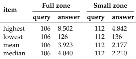
The open and verified resolvers are queried for a large zone to get the approximate maximum message size that the resolvers can send. The DNS measurement domain (dnsscan.zkkd.nl) is setup with TXT records resulting in an answer of approximately 3.800 bytes. This domain or zone is called ’full zone’ throughout the thesis. The same scan results are used for the bandwidth estimation in Section5.2. The scan is repeated for a smaller zone (dnsscan-small.zkkd.nl) for the resolvers that couldn’t provide the answer to the previous query. This smaller domain or zone is called ’small zone’ throughout the thesis. The smaller zone is setup with TXT records re-sulting in an answer of approximately 2.100 bytes. This smaller zone is still large enough to cause packet fragmentation, since theMaximum Transmission Unit(MTU)

is 1.500 bytes according to the standard [16]. The query and answer size for both the resolvers that successfully answered the query and the resolvers that failed to answer the query is measured. This is done by sending a query to the resolvers using dig and monitoring the output for a successful or failed answer. Parameters are passed to dig to force the use of UDP as transport layer protocol, and truncated answers are not retried using TCP. At the same time tcpdump is started to capture the network traffic going in and out of the measurement machine. The payload size of the packets of fragmented answers is summed, based on source and destination IPv6 address of the packet. The frame length of the packet is used as the payload size, this has the protocol headers of UDP and IPv6 included in the size.

(31)

Chapter 5. Performance Quantification of Open DNS Resolvers 23

item Full zone Small zone query answer query answer

highest 106 8.502 112 4.842

lowest 106 126 112 136

mean 106 3.923 112 2.177

median 106 4.040 112 2.210

TABLE5.1: The highest, lowest, mean and median value, in bytes, of

the message size of the successful queries

item Full zone Small zone query answer query answer

highest 1.400 4.343 1.406 4.238

lowest 106 66 112 66

mean 113 309 116 311

median 106 106 112 112

TABLE5.2: The highest, lowest, mean and median value, in bytes, of

the message size of the failed queries

is twice the size of the zone, about 8.000 bytes for the full zone of 3.800 bytes. The reason is that those resolvers answered the single query twice. This could be because of a flaw in the resolver’s software or something happened during the transportation of the query or answer. It is also possible that some resolvers forward the query to another resolver that in turn processes the query and sends the answer back. This means that two front-end resolvers use the same back-end resolver to answer the query, or one resolver forwards the query to a second resolver. Since filtering is used during the data processing, the resolver answering the queries must also exist in one of the IPv6 address sources and also received a query during the scanning. The open DNS resolvers failing the query, return 0 answers and the rcode of SERVFAIL or refuse to preform a recursive query. The measured message size in bytes for the query and answer of the resolvers failing to resolve the query of the full zone and the small zone, is shown in Table5.2. The reason that the message size is still significant, is that some resolvers return the A, AAAA and NS records of the root nameservers. From the resolvers failing the query for the full zone, 78 return an answer that is 1.000 bytes or larger, for the small zone this is 57 resolvers. There are even 2.172 resolvers that return an answer that is 600 bytes or larger for the full zone, for the small zone this is 2.179 resolvers.

A normal query for the full zone is 106 bytes and the small zone is 112 bytes. The table however, shows that query sizes of 1.400 and 1.406 also occur. The reason is that some answers couldn’t be reassembled within the reassembly timeout. This causes the measurement machine processing the answer to send an ICMP Time Exceeded message to the resolver. This ICMP packet is captured by tcpdump and added to the message size of the query.

Figure5.1shows a plot of the answer size for all the resolvers mentioned above. The plots of the full and small zone of successful answers are almost the same. The difference is that a small number of resolvers managed to resolve the small zone, but not the full zone. This is probably because the larger payload doesn’t fit in the

[image:31.595.174.397.82.179.2]

(32)

0 500 1000 1500 2000 2500 3000 3500 4000 resolvers 0 1000 2000 3000 4000 5000 6000 7000 8000 9000 answer size [bytes]

Full zone successful answers

0 500 1000 1500 2000 2500 3000 3500 4000 4500 resolvers 0 1000 2000 3000 4000 5000 answer size [bytes]

Small zone successful answers

0 1000 2000 3000 4000 5000 6000 7000 8000 9000 resolvers 0 500 1000 1500 2000 2500 3000 3500 4000 4500 answer size [bytes]

Full zone failed answers

0 1000 2000 3000 4000 5000 6000 7000 8000 resolvers 0 500 1000 1500 2000 2500 3000 3500 4000 4500 answer size [bytes]

Small zone failed answers

Answer message size

FIGURE5.1: Answer message size in bytes of the query to the open

resolvers of the IPv6 address list

to resolve the query and return a SERVFAIL rcode. The same difference can be seen between the failed answers of the full and small zone. The full zone has a little more failed answers than the small zone has.

Overall the successful answers are relatively constant. There is however, a valley at beginning and a peak at the end of the graph. The valley at the beginning indicates a number of resolvers not able to return all the TXT records requested for, but only a single A or AAAA record. This still sets the number of answer records in the answer, so passes the successful/fail test. The peak at the end of the graph indicates a number of resolvers that responded twice to a single query. That is also why the graph is about twice as high there.

The failed answers are consistent in the beginning. Most of these resolvers don’t support recursion, thus reply with an empty answer or a small answer pointing to the root DNS servers. There are also some resolvers that could not answer the query for the large zone, thus replied with a SERVFAIL rcode and a small or empty answer. The increase in message size after that indicates the resolvers that refuse to answer recursive queries, but reply with a relatively large answer with A, AAAA or NS records of the root DNS servers. The peak in message size at the end of the graph has multiple causes. The resolver could actually have resolved the zone, but the answer is received after the timeout of the query, which is 16 seconds, twice as long as zmap uses. The answer is thus added to the tcpdump capture and processed, but ended up in the failed answers. Another cause is that a fragment is lost, or not send by the resolver. This way the packet cannot be reassembled, thus no answer is received. But the answer is added to the tcpdump capture, just like above.

5.1.2 Amplification Factor

(33)

0 500 1000 1500 2000 2500 3000 3500 4000 resolvers 0 10 20 30 40 50 60 70 80 90 amplification factor

0 500 1000 1500 2000 2500 3000 3500 4000 4500 resolvers 0 5 10 15 20 25 30 35 40 45 amplification factor

0 1000 2000 3000 4000 5000 6000 7000 8000 9000 resolvers 0 5 10 15 20 25 30 35 40 45 amplification factor

0 1000 2000 3000 4000 5000 6000 7000 8000 resolvers 0 5 10 15 20 25 30 35 40 amplification factor

Small zone failed answers Amplification factor frame.len

FIGURE5.2: Amplification factor with the frame length as message

size

also be used, as it is the actual length of the data without the Ethernet headers ap-pended to it. The amplification factor will be even greater if the application layer message size is used. The IPv6 and the UDP headers are excluded then. The UDP header takes another 8 bytes on top of the IPv6 header. So the amplification factor for the application layer message can be calculated by subtracting 8 from the query and answer message size. It’s assumed that the amplification factor correlates to the message size of the answer of the DNS query that is send to the resolver. This is be-cause the message size of the query itself is the same to all resolvers. It will however, not be entirely the same for the failed resolvers. That is because the measurement machine sending the queries, is sending ICMP messages to some resolvers that sent fragmented answers that could not be reassembled within the reassembly timeout, as is mentioned in5.1.1. Rate limiting can be applied to DNS resolvers to prevent rapid querying of the resolvers. However, research conducted by MacFarland et al. [24] found that only 149 (2.69%) of studied name servers employed rate limiting. This means that for nearly all the found open DNS resolvers, the amplification fac-tor can be achieved when repeatedly querying the resolvers. This could of course be verified by repeatedly querying all the resolvers, but for ethical reasons this not performed.

The amplification factors of the resolvers with the frame length as message size, are shown in Figure5.2. The average amplification factor of the resolvers resolving the full zone, with an answer size of approximately 3.800 bytes, is a bit less than 40. For the small zone the amplification factor is a little bit less than 20. The same peak and valley as in the message size plot can be seen. This is because the query size is for every resolver the same, and a smaller answer size corresponds to a smaller amplification factor. The resolvers that send the answer twice have an amplifica-tion factor about twice as high. The highest, lowest, mean and median value of the amplification factor is shown in Table5.3

(34)

item Successful Failed

full zone small zone full zone small zone

highest 80.2 43.2 41.0 37.8

lowest 1.2 1.2 0.4 0.4

mean 37.0 19.4 2.8 2.8

median 38.1 19.7 1.0 1.0

TABLE5.3: The highest, lowest, mean and median value of the

am-plification factor, with frame-len as message size

0 500 1000 1500 2000 2500 3000 3500 4000 resolvers 0 20 40 60 80 100 120 140 160 amplification factor

0 500 1000 1500 2000 2500 3000 3500 4000 4500 resolvers 0 10 20 30 40 50 60 70 80 amplification factor

0 1000 2000 3000 4000 5000 6000 7000 8000 9000 resolvers 0 10 20 30 40 50 60 70 80 amplification factor

0 1000 2000 3000 4000 5000 6000 7000 8000 resolvers 0 10 20 30 40 50 60 amplification factor

Small zone failed answers

Amplification factor ipv6.plen

FIGURE5.3: Amplification factor with the IPv6 payload size as

mes-sage size

zone, with an answer size of approximately 3.800 bytes, is a bit less than 75. For the small zone the amplification factor is a little bit more than 35. The same peak and valley as in the message size plot can be seen. This is because the query size is the same for every resolver, and a smaller answer size corresponds to a smaller amplification factor. The resolvers that send the answer twice have an amplifica-tion factor about twice as high. The highest, lowest, mean and median value of the amplification factor is shown in Table5.4

For the complete picture, the amplification factor calculated with the message size of the packets at the application layer, is shown in Table5.5. This results in the highest amplification factor since all the UDP and IPv6 headers aren’t in the calcu-lation. The resulting amplification will not be achieved, since the packet headers mentioned above are send on the wire. But this amplification factor is achieved when looking only at the DNS protocol information.

5.1.3 Types of Resolver Addresses

(35)

highest 155.2 79.8 79.4 50.6

lowest 1.4 1.4 0.2 0.2

mean 71.8 35.7 4.8 4.4

median 73.5 36.2 1.0 1.0

am-plification factor, with ipv6-plen as message size

highest 183.2 92.4 93.6 58.5

lowest 1.5 1.5 0.1 0.1

mean 84.7 41.3 5.4 4.9

median 86.7 41.9 1.0 1.0

ampli-fication factor, with the message size of the packets at the application layer

the two halves of the MAC address. Then the 7th bit of the IID is complemented (i.e., ’flipped’). Thus the resulting address consists of the network prefix and the IID. For example, the MAC address ’12:34:56:ab:cd:ef’ and the network prefix ’2a02::’ results in the IPv6 address: ’2a02::1034:56ff:feab:cdef’.

The second type of IPv6 is a ’seemingly random address’. An IPv6 address is classified as seemingly random if the IID part of the IPv6 address has a hamming weight (number of bits set to ’1’ in the IPv6 address) of 16 or less. The average ham-ming weight of an IID of an IPv6 address is 32, since the length of the IID is 64 bits. By looking at the hamming weight, the second address type can contain addresses from SLAAC with privacy extensions, manually configured addresses with at least 16 bits set to ’1’ or addresses created in a different way. SLAAC with privacy exten-sions randomizes the values after the network prefix [28], the IID. The address ran-domization can be achieved using different techniques, divided in two cases based on whether stable storage is present. When stable storage is present, the randomized IID is created using a number of steps. First the history value from the previous iter-ation is used if it’s available, or a random value is generated. Then the MD5 message digest is computed over the random value. The leftmost 64-bits of the MD5 digest is used, and 7th bit of that value is set to zero. This creates an interface identifier with the universal/local bit indicating local significance only. The rightmost 64-bits of the MD5 digest are stored in the history value to be used for the next iteration. In the absence of stable storage, a random number is generated every iteration. An alternate approach isCryptographically Generated Addresses(CGA), which generate a

random IID based on the public key of the device. In case DHCP is used to generate a random looking address, the address is categorized in this address type.

(36)

address type amount of resolvers percentage

SLAAC 1.288 10.4

Seemingly random (hw > 16) 1.227 9.9

Manual (hw <= 16) 9.829 79.6

Total 12.344 100

TABLE 5.6: Open and verified resolvers: IPv6 address types where

’hw’ means the hamming weight of the interface identifier part of the IPv6 address

non-zero values amount of resolvers percentage

Only in last hextet 13.429 68.3

Also other hextets 6.224 31.7

Total Manual addresses 19.653 100

TABLE5.7: Open and verified resolvers: non-zero values in the last hextet of the IPv6 address or also in other hextets

machine is encoded in its IPv6 address, like ’::53’ for a DNS resolver.

For all the open and verified resolvers, the IPv6 address type is shown in Table

5.6. As can be seen from the table, most of the resolvers have manually configured IPv6 addresses. Which is interesting, since these addresses are manually set up by administrators for a specific purpose, in this case DNS resolving. For the manual assigned IPv6 addresses, whether only the last hextet of the IPv6 address contains non-zero values, or also other hextets, is shown in Table5.7. The hamming weight of the IIDs of the open and verified resolvers is shown in Figure5.4. The blue line represents the hamming weight of the IIDs of the IPv6 addresses. The red line rep-resents the hamming weight of randomly generated IIDs, where there are generated as many IIDs as there are IIDs represented by the blue line. As can be seen, the normal hamming weight should be around 32, where the IID has a length of 64 bits. The blue line indicates that the majority of the addresses have more zeros than ones. Even though the SLAAC addresses have ’fffe’ in the IID, which has a hamming weight of 15 out of the 16 bits.

Discovery and Quantification of Open DNS Resolvers on IPv6

U

NIVERSITY OF

T

WENTE

M

T

Discovery and Quantification of Open

DNS Resolvers on IPv6

Abstract

Contents

List of Figures

List of Tables

List of Abbreviations

1 Introduction

1.1

Domain Name System

1.2

DNS Resolvers

1.3

Research Questions

1.4

Research Approach

2 Related Work

2.1

Finding Open DNS Resolvers

2.2

Performance Quantification

3 Methodology

3.1

Finding Open DNS Resolvers

3.2

Performance Quantification

4 Discovery of Open DNS

Resolvers

4.1

IPv6 Address Sources

4.2

Scanning on the Full Data Set

4.3

Validation of the Full Data Set

4.4

Results of the Scanning and Validation

5 Performance Quantification of

Open DNS Resolvers

5.1

Classification of Open DNS Resolvers