Robust estimation of biometric data

(1)

Robust Estimation of Biometric Data

Guido Kuijper

Abstract: This study presents the design of a robust estimator ˆC to apply on biometric data analysis involving facial recognition. This functional estimates the covariance matrix of a multivariate Gaussian distribution by seperately estimating the matrix elements. It is first mathematically derived, then classified by means of its efficiency at Gaussian distributions and finally applied to both synthetic and real biometric data. The synthetic experiments show the ˆC-estimator performs in between the sample covariance and the MCD estimator. The test with the real data shows clear improvement of the robust ˆC-estimator as it was able to link two faces for which the sample covariance estimator was not able to.

1 Introduction

Nowadays one of the fields that employ statistical methods the most is the field of biometrics. This application is referred to as biostatistics and within biometrics, biostatistics is often applied to genetical data to model the influence of groups of genes. [1] Another application of biostatistics is in the field of computer vision and in particular the field of facial recognition. This paper complements the method presented in Spreeuwers [2] and improved in Spreeuw-ers [3]. These papSpreeuw-ers use a classifier based distinction between the classes and class members, where it is assumed both the classes and members of a class are normal distributed.

The covariance matrices of these multivariate dis-tributions are estimated, which are then used in a LDA-based classification. The estimation of covari-ance matrices is notoriously susceptible to outlier interference [4]. To solve this problem, one can turn torobust statistics. This branch deals with outliers and corrupted data. Robust estimation has seen a good amount of mathematical development start-ing from Hampel [5], who defined the concept of robustness from the influence function, called the influence curve back then, and some measures that can be derived from it. A public start on the ro-bust estimation of covariance matrices was made by Gnanadesiken and Kettenring [6]. Maronna [7] was the first to formulate robust M-estimators in this con-text. Subsequently many approaches to this problem were described, including theminimum determinant covariance (MCD) [8], projection methods [9] and computing the smallest volume ellipsoid over the set of data [10].

Overview : This paper starts with a short overview of important definitions in robust statistics in section 2, the description of the often-used MCD estimator in section 3 and in section 4 the design of the ˆC-estimator is presented. Then in section 5 experiments are done with synthetic data that model often occuring con-taminations in facial datasets. A score evaluation of real facial data can be found in section 6. The paper ends with a discussion of the results in section 7.

2 Robust Statistics

This section was written as a summary of Hampel et al [11], with the intention of introducing some im-portant concepts that are going to be discussed in this paper. One of the most important definitions in robust statistics is the definition of theinfluence function (IF).

Definition : The influence function of functional T at distribution F is given by:

IF(x;T, F) = lim

t→0

T((1−t)F+t∆x)−T(F)

t

The influence function is therefore a directional direc-tive from T at F to T at ∆xwith the latter denoting

the probability measure that puts mass 1 at the point x. Heuristically, the interpretation of the influence function is that it is a quantity of how much the estimator T becomes corrupted when sample x is con-tamined with ∆x.

(2)

Definition : The gross-error sensitivityγ of a func-tional T at distribution F is given by:

γ(T, F) = sup

x

|IF(x;T, F)|

If this quantity is finite, we call the estimator B-robust at F. Intuitively, this means no contamination at any sample results in an unbounded error in the estima-tion. It is a desirable property for an estimator to be B-robust.

Theorem : The asymptotic variance of T at F equals:

V(T, F) =

Z

IF(x;T, F)2dF(x)

This gives a way to quantify the variance of the es-timator in the asymptotic domain, which relies on the notion of the influence function. The asymptotic variance is bounded by the inverse of the Fisher infor-mation. The Fisher information is defined as: Definition : The Fisher information at Fθ equals:

IF(fX,θ) =

Z

fX,θ(x)

_∂_ln_f

X,θ(x)

∂θ

2

dx

It provides a measure of how much information a random variable carries of a parameterθthat its dis-tribution depends on.

The fundamental bound of the asymptotic variance is given by the Cramer-Rao inequality:

V(Tθ, F)≥

1 IF(fX,θ)

Using this bound, we can define the asymptotic effi-ciency of an estimator:

Definition : The asymptotic efficiency of an estima-tor T of a parameter θat distribution F is given by: Eff = (V(T,F)IF(fX,θ))−1.

Lastly we have an independent quantity named the maximum breakdown point (p). This is the maximum amount of observations before the estimation can go arbitrarily wrong. Intuitively it makes sense that p can never be greater than 0.5, as in that case the outliers would be considered the data.

3 MCD Estimator

Definition: Consider a set of data X = [x1, ..., xn]

with each xi consisting of p different observations.

Therefore X is a n x p matrix. Using this dataset we can derived the Malahanobis distance [12] which is defined to be the set of p-dimensional points which satisfy:

M D(x) =p(x−x)¯ t_S−1_(x₋_{x) =}_¯ q_χ2 p,0,975

Where ¯x is the sample mean and S the sample co-variance. Withχ2_α theα-quantile of the chi-squared distribution is meant.

The MCD has a parameter h. For the h observa-tions that minimize the determinant of the sample covariance matrix S, we can derive two estimates:

1. ˆµ0 is the sample mean of thesehobservations.

2. ˆΣ0 is the corresponding covariance matrix

(mul-tiplied with a scalar to be consistent). These estimates yield another distance metric:

di =

q

(x−µˆ0)tΣˆ0−1(x−µˆ0)

This distancedi is then used to find the MCD

esti-mates for location and scatter: ˆ

µMCD =

Pn

i=1W(d 2 i)xi

Pn

i=1W(d 2 i)

ˆ

ΣMCD = c

1 n

n

X

i=1

W(d2_i)(xi−µˆMCD)(xi−µˆMCD)t

The constant c is for consistency.

W is a weighting function and is defaulted to W(d2_{) =}_I_d2_≤q_χ2

p,0,975

in MATLAB [8].

(3)

efficiency for Gaussian distribution decreases if β in-creased. However, for increasing amounts of observa-tions p, the efficiency rises. They proved for the MCD estimator:

lim

p→∞Eff( ˆΣMCD,ij,Φ) = 1−β ∀i≥1, j≤p

In addition, it was shown that a class of estimators, which include ˆΣMCD, have asymptotically the same

properties as [14]. Lastly, the FAST-MCD algorithm was developped by Rosseeuw and Van Driessen [15]. This theoretical clarity and application support of the MCD estimator make it an attractive choice.

4 C

ˆ

-Estimator

A second choice for a robust estimator of covariance is the ˆC-estimator. This estimator was proposed by Gnanadesikan and Kettenring [6]. They propose to estimate each seperate element in the covariance ma-trix based on the following identity, valid for random variables X and Y:

Cov(X, Y) = 1

4(var(X+Y)−var(X−Y)) By plugging in a robust estimator of scale, denoted byS(X), we can estimate each covariance by:

ˆ

C(X, Y) = 1

4 S(X+Y)

2₋_S(X₋_Y₎2₎

This estimator has some problems:

• A covariance matrix is necessarily positive-semidefinite [16]. However this estimator does not automatically produce a positive-semidefinite matrix. Therefore the shape el-lipsoid may be hyperboloid.

• As far as the author knows, no robustness prop-erties have been derived for this estimator. The rest of this section is devoted to solving these problems:

Conditioning theC-estimatorˆ : A covariance ma-trix is only positive semi-definite if one of the random variables is linearly dependent on another. Therefore, for data where one does not expect linear dependence between samples, we will introduce a scheme to en-force a positive definite (PD) covariance matrix. We use the following theorem, by Sylvester [17]:

Theorem 1. : A matrix M∈Rnxnis PD if and only

if all of its principle minors are PD and det(M) >0. This theorem is also called Sylvester’s criterion. This criterion is used to build the matrix in a way that resembles mathematical induction:

Theorem 2. : A matrix M∈R1x1is PD if and only

if det(M)>0.

The covariance matrix of a single variable X is given by the variance of X or cov(X,X). As cov(X,X)>0, a covariance matrix of one variable is always PD. Now suppose we have n variables and the covari-ance matrix of p variables with p < n is given by Ap∈Rpxp and det(Ap)>0. We have then that the

covariance matrix of p+1 variables has the following form:

ˆ Σp=

A B

BT D

With ˆΣp the sample covariance matrix of p+1

vari-ables. B is given by ˆC(Xi, Xp+1)∀i < p+ 1 and B

is given by ˆC(Xp+1, Xp+1), T denoting the transpose.

Notice that if det( ˆΣp)>0, the estimated covariance

matrix will be PD.

For the determinant of a matrix M, the following identity is the case:

det

A B

C D

= (D+ 1)·det(A)−det(A+BC) ForC=BT we have an expression for det( ˆΣp).

An-other determinant identity, also by Sylvester [18], is as follows:

det(A+BC) = det(A)·det(Im+C·A−1·B)

ForC=BT _{we substitute this identity in 4, obtaining:}

det( ˆΣp) = det

A B

BT _D

= det(A) (D+ 1)−det(Im+BTA−1B)

We require det( ˆΣp)>0. Therefore the following

in-equality needs to hold:

det(A) (D+ 1)>det(A)det(Im+BTA−1B)

(4)

AsB is a row vector andBT _{a column vector, we are}

taking the determinant over a number, which is the number itself:

(D+ 1)>1 +BTA−1B→D > BTA−1B Therefore if we multiple D with a scalar c, we can enforce our estimated matrix to be PD. We lose unbi-asedness for the diagonal elements of the however. By minimizing c, this problem can be partially circum-vented.

Robustness properties of the C-estimatorˆ To establish robustness properties, as suitable candidate for the robust scale estimator S(x) has to be defined first. An attractive candidate is theQn estimator, as

described by Rosseeuw and Croux [19]. Qn=d(|xi−xj|;i < j)_(k)

Wherexi, xj are samples , (k) denotes the k-th order

statistic and d is a consistency factor equal to 2.2219 at Gaussian distributions.

This estimator was shown to have a breakdown point of 50% of the samples. Additionally, it has an efficiency at Gaussian distributions of 82.27%. The functional of this estimator at a distribution F is given by:

Q(F) = inf

s >0;

Z

F(t+d−1s)dF(t)≥5/8

The influence function of the estimator at distribution F is given by:

IF(x;Q, F) =d1/4−F(x+d

−1_{) +}_F(x₋_d−1₎

R

f(y+d−1_)f_(y)dy

Withf the density of F.

This influence function describes a smooth curve. Now the ˆC-estimator can be defined as follows:

ˆ

C(X, Y) = 1 4

Qn(X+Y) 2

−Qn(X−Y) 2

To establish robustness properties of the ˆC-estimator, we will need to establish its influence function. The es-timator is dependent on two different variables, which means that we have to determine thepartial influence functions instead, denoted by PIF(x; T, F). These

partial influence functions were introduced by Hampel et al [11] in the form of influence functions for tests. Partial influence functions in their current form were defined by Pires and Branco [20] However, the partial influence functions PIF(x;Qn,F) and PIF(y;Qn,F) are

hard to directly evaluate, asQn is not linear.

There-fore we will perform a change of variables: let Z = X + Y and W = X - Y. The ˆC-estimator now reads as

follows: ˆ

C(X, Y) =1

4 Qn(Z(X, Y))

2₋_Q

n(W(X, Y))2

Notice Z and W are normally distributed.

IfX, Y ∼N(0,1),Z ∼N(0, σ+) andZ ∼N(0, σ−).

Here σ± =

p

2±2·cov(X, Y). As the influence function is special case of a Gˆateaux derivative [21], we are allowed to use the chain rule if the influence function is continuous. Therefore:

P IF(z; ˆC, Fz) =

1

2 ·Q(Fz)·IF(z;Qn, Fz) P IF(w; ˆC, Fw) = −

1

2 ·Q(Fw)·IF(w;Qn, Fw) Where Q(F) denotes the estimator functional acting on a distribution F.

Both partial influence functions are B-robust, as the gross-error sensitivity is finite.

Theorem 3. : γ( ˆC,Φ) = supx|P IF(x; ˆC,Φ)| and

γ( ˆC,Φ) = supy|P IF(y; ˆC,Φ)|are finite.

Proof. : As z = x+y is normally distributed, _σz + is distributed N(0,1), therefore P IF(x+y_σ

+ ; ˆC,Φ) = P IF(z; ˆC, Fz). As the latter is a bounded function,

set x = 0 or y = 0.

Intuitively this is correct, since P IF(z; ˆC, Fz)

con-sists of possible point contaminations in x or y, but any point contamination will be the same as a point contamination in z.

Asymptotic Properties : As we aim to evaluate the ˆC-estimator for the standard normal distribution Φ, we need a change of variables. In a way analogous to the proof of 3, it can be seen that z

σ+ and

w σ− are

(5)

Using this change of variables, we obtain:

P IF

_z

σ+

; ˆC,Φ

= 1

2·Q(Φ)·IF

_z

σ+

;Qn,Φ

P IF

_w

σ−

; ˆC,Φ

= −1

2 ·Q(Φ)·IF

_w

σ−

;Qn,Φ

Note thatQ(Φ) = 1 so it is no longer considered in the derivation.

We use the definition of asymptotic variance as given by Pires and Branco [20] which is to be evaluated for the ˆC-estimator at a standard normal distribution for X and Y, with the additional case that we have as many samples for X as for Y:

V(c; ˆC,Φ1,Φ2) = 2·V1(c; ˆC,Φ1,Φ2)

+2·V2(cov; ˆC,Φ1,Φ2)

Where the partial asymptotic variancesVi are given

by:

Vi(c; ˆC,Φ1,Φ2) =

Z

IFi(x; ˆC,Φ1,Φ2)2dΦi(x)

We end up with the following expression for the asymp-totic variance:

V(c; ˆC,Φ1,Φ2) =

1 2

Z

IF

_z

σ+

; ˆC,Φ

2

dΦ

_z

σ+

+1 2

Z

IF

_w

σ−

; ˆC,Φ

2

dΦ

_w

σ−

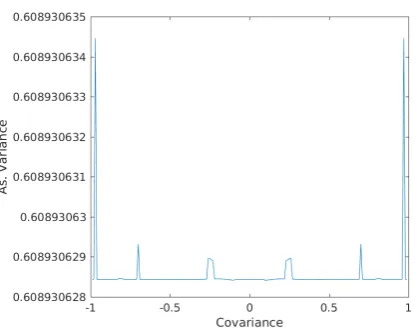
V can now be evaluated with help of numerical integra-tion. Notice that V in fact depends on the covariance that is being estimated. Therefore we now have to plot V versus the covariance. This plot can be found in figure 1. By a probatilistic corollary of the Cauchy-Swartz inequality, we have:

|Cov(X, Y)|2_≤_Var(X₎_·_Var(Y₎

Since we are seeking the variance at Φ, the variances of X and Y are 1 and−1≤Cov(X, Y)≤1.

The asymptotic variance appears to be almost con-stant over the whole covariance spectrum. The value is about 0.6089, which is very close to the asymptotic variance of Qn as reported by Croux and Rosseeuw

[image:5.595.305.513.114.280.2]

[19].

Figure 1: Asymptotic Variance versus Covariance

To evaluate the efficiency at Gaussian distributions, a different kind of Fisher information is required: the joint Fisher information [22]. This quantity is depen-dent on the joint density functionfX,Y(x, y) and the

parameter Θ. It is defined to be:

IF(fX,Y,Θ) =

Z Z

X,Y,Θ

(x, y)

_∂_ln_f

X,Y,Θ(x, y)

∂Θ

2

dxdy

In our case, the parameter Θ is given by Cov(X,Y). Note that Cov(X,Y) = Cov(Y,X). Since the Fisher in-formation gives a score of the amount of inin-formation a random value carries about an unknown parameter Θ, an observable value in this case carries twice as much information since it has a score on Cov(X,Y) and on Cov(Y,X). The efficiency at Gaussian distributions is then given as follows:

Eff(c; ˆC,Φ,Φ) = 1

2IF(fX,Y,Cov(X,Y))V(c; ˆC,Φ1,Φ2)

(6)

[image:6.595.73.276.116.281.2]

Figure 2: Gaussian Efficiency versus Covariance

This can be numerically solved as well and figure 2 is obtained. We see that the ˆC-estimator has a high efficiency for low covariance (82.11% at the peak) but quickly loses efficiency when estimating higher covari-ances. 82.11% is very close to the Gaussian efficiency of the Qn estimator, which sits at 82.27%. By

remov-ing the strange peaks from figure 1, we get a peak efficiency of 82.28%.

5 Sample Asymptotic Variance

In the context of facial recognition, we would like to find out the performance of the MCD- and ˆ C-estimators in comparison to the normal sample co-variance matrix S. To obtain this knowledge, various experiments with synthetic data have been performed. In lieu of the synthetic data portraying as actual facial data, the PD-enforcing scheme has not been utilised. This has four reasons:

1. Facial data often contains pixels that are lin-early dependent on their neighbour pixel, espe-cially at the edges of the pictures. This results in the actual covariance matrix being positive semi-definite instead of positive definite. A PD-enforcing scheme could therefore distort the es-timation quite heavily.

2. Facial data generating positive semi-definite ma-trices result in determinants of zero, which there is no inverse, which is needed for the scheme.

This can be circumvented by taking Moore-Penrose pseudo-inverses [23], however when the author attempted this work-around, the matrix remained singular to working precision. 3. The scheme requires more processing time. 4. Lastly, in none of the synthetic datasets that

pa-rameters were estimated from, did it occur that the diagonal elements had to be changed. No case was noted where the ˆC-estimator did not generate a positive (semi)-definite covariance matrix.

In this experiment, we attempt to simulate possible dataset errors. The first of these is simply a collec-tion of random outliers, which happen if for example a rogue picture finds its way in the database. The second kind of error that is simulated is an different distribution that is mixed through the data that is to be estimated. This happens if for example a series of pictures is taken with bad lighting.

We ask the following questions that we hope to an-swer with the two fprms of simulations of database contamination:

1. Will the C-estimator perform worse underˆ higher covariance? Figure 2 predicts worse re-sults if the covariance is higher. To test this, we will use 100 datapoints and 10 outliers. The out-liers are there because the the sample covariance is optimal otherwise and we are interested in robust estimation. We will subsequently higher the covariance from 0 to 0.5 to 0.99.

2. Will the MCD estimator perform worse under influence of more outliers, as predicted by Croux and Haesbroeck [13]. We use the outlier distri-bution to answer the question, as in reality, one is more likely to encounter a large amount of similarly contaminated samples than encounter a database with many single outliers.

(7)

5.1 Single Outliers Set-Up

The first synthetic test was withnrandomly gener-ated data following a normal distribution N(0,1) with covariance 0. Then out outliers were added to the total data, the outliers were generated as points on a circle with radius R. Then the covariance matrix was determined in three different ways:

1. The sample covariance S 2. The MCD covariance ˆΣMCD

3. The ˆC-estimator covariance ˆC.

This process was repeated 100 times, every time with new random data and new outliers. The average of the covariance matrix elements are shown below, as are their variances.

Values: n = 100, R = 10 and out = 10.

Table 1: S Average 5.94 0.02 0.02 5.02

Table 2: S Variance 0.02 0.01 0.01 0.02

Table 3: ˆΣMCD Average

1.15 0.03 0.03 1.12

Table 4: ˆΣMCD Variance

0.05 0.02 0.02 0.05

Table 5: ˆC Average 1.44 0.03 0.03 1.32

Table 6: ˆC Variance 0.05 0.02 0.02 0.06

Values: n = 100, R = 20, out = 10.

Table 7: S Average 21.06 -0.02 -0.02 17.44

Table 8: S Variance 0.02 0.01 0.01 0.01

1.15 -0.03 -0.03 1.17

0.05 0.02 0.02 0.04

Table 11: ˆC Average 1.50 -0.04 -0.04 1.34

Values: n = 100, R = 30 and out = 10.

Table 13: S Average 46.27 -0.004 -0.004 38.05

Table 14: S Variance 0.02 0.01 0.01 0.02

1.18 0.00 0.00 1.13

0.05 0.02 0.02 0.04

Table 17: ˆC Average 1.54 0.01 0.01 1.32

Then the non-diagonal elements of the actual covari-ance are varied to 0.5 and then to 0.99, since 1 will give a singular matrix. Values: n = 100, µ = 0, Σ =

1 0.5 0.5 1

, out = 10.

Table 19: S Average 5.96 0.47 0.47 5.08

Table 20: S Variance 0.02 0.01 0.01 0.02

1.16 0.59 0.59 1.18

(8)

Table 23: ˆCAverage 1.47 0.73 0.73 1.38

Table 24: ˆCVariance 0.05 0.03 0.03 0.06

Values: n = 100, µ = 0, Σ =

1 0.99 0.99 1

, out = 10.

Table 25: S Average 5.95 0.90 0.90 5.04

Table 26: S Variance 0.02 0.02 0.02 0.02

1.16 1.15 1.15 1.16

0.05 0.05 0.05 0.05

Table 29: ˆCAverage 1.45 1.40 1.40 1.37

Table 30: ˆCVariance 0.06 0.06 0.06 0.06

5.2 Outlier Distribution Set-Up

To simulate contamination of the database with an-other set of data, we will once again vary the amount of outliers, but this time they are distributed following N(µout,Σout).

Values: n = 100, µout = (5,5), Σout =

1 0 0 1

, out = 10.

Table 31: S Average 3.07 2.11 2.11 3.11

Table 32: S Variance 0.11 0.05 0.05 0.08

1.14 0.00 0.00 1.14

0.04 0.01 0.01 0.04

Table 35: ˆC Average 1.47 0.23 0.23 1.44

1 0 0 1

, out = 20.

Table 37: S Average 4.54 3.52 3.52 4.51

Table 38: S Variance 0.17 0.06 0.06 0.18

1.31 -0.01 -0.01 1.33

0.05 0.02 0.02 0.07

Table 41: ˆC Average 1.98 0.49 0.49 2.01

1 0 0 1

, out = 40.

Table 43: S Average 6.12 5.13 5.13 6.11

Table 44: S Variance 0.11 0.06 0.06 0.15

1.74 0.01 0.01 1.73

0.08 0.04 0.04 0.08

Table 47: ˆC Average 3.07 1.04 1.04 3.06

(9)

6 Real Data Test

Spreeuwers [3] designed a classifier to decide if a probe sample X belongs to the same class ci as a gallery

sample Y. This classifier uses linear discriminant analyses (LDA) [24] as well as principle component analysis (PCA). The classifier needs a within-class-meanµw, atotal-mean µtand awithin-class andtotal

covariance matrix respectively denoted as CwandCt.

From these matrices and vectors, a statistic is derived that assigns a value to the samples X and Y. It is also possible to enter more probe samples or more gallery samples or both. If the statistic has a value above 1, the chance that the samples are from the same class is higher than the opposite and vice-versa for a value below 1. If the statistic assigns 1, the chance that the samples are from the same class is just as high as the chance that they are not.

The test: 100 pictures were taken from a database, of which 1 was an obvious outlier. These pictures had 87x75=6525 pixels ranging from 0 to 255 depending on their black-white scale. These 100 pictures were used to determine two covariance matrices to estimate Ct, one normal sample covariance matrix and the

other the matrix generated by the robust ˆC-estimator. Remark: it took 8 hours to process the robust estima-tor. There exists a faster algorithm for the estimation ofQn made by Croux and Rosseeuw [25]. The author

recommends using this version, it improves the time from O(n2_{) to O(n log(n)). Remark 2: The}

MCD-estimator was not used here as the code required too many samples.

Then a selection of 20 pictures was made, 19 of which belonged to the same person and 1 obvious outlier. These 20 pictures were used to estimateCw. Similarly

to estimating Ct, there were a robust version and a

non-robust version of this covariance matrix too. In addition, anywhere where a location estimate was needed, the median was used.

Subsequently, 2 pictures of the same person were fed to the classifier, one as the probe and one as the gallery. The classifier first assigned a score on basis of the non-robust covariance matrices, then assigned a score on basis of the robust covariance matrices. Result: The score, using non-robust matrices: 0.00459. Using robust matrices: 1015.98.

7 Discussion

The theoretical part of the paper had 4 main results: 1. Conditioning the estimate to become PD; 2. Proving the ˆC-estimator is B-robust;

3. Evaluating the asymptotic variance of the ˆ C-estimator at Gaussian distributions;

4. Evaluating the Gaussian efficiency of C-ˆ estimator.

The first result does not carry a lot of importance: as discussed in section 5, it is not very useful in the context of facial recognition. However the result is still valid for possible other cases where an estimate has to be PD and the statistician is willing to let go of unbiasedness for the diagonal elements.

The second result is necessary to even consider using the ˆC-estimator. Without robustness properties, we shall not consider it as a candidate. What this result is still lacking however is a concrete value for the gross-error sensitivity to see exactly how well the estimator resists point mass contaminations. This is still an open question.

The third result is in agreement with the findings of Croux and Rosseeuw. We can conclude that we can build a robust estimator that achieves a V( ˆC,Φ) of 0.6089 for every covariance and not only for variance alone. It is worthwhile to research further applications of this estimator. The small peaks are a bit strange, the author suspects numerical computing errors, but for a flatlined asymptotic variance, the results fully agree with Croux and Rosseeuw.

The fourth result has room for interpretation. For un-correlated random variables X and Y, the ˆC-estimator is virtually the same asQn as it can estimate their

variances with the same high efficiency. However, as soon as X and Y become correlated, the efficiency drops heftily and the estimator becomes fairly weak. This partially has to do with very high values for the Fisher information on covariances that go to 1 or -1. On the topic of the Fisher information, it turned out we had to consider Cov(X,Y) but also Cov(Y,X). It evokes a question if we have to consider all parameters Θi that have the same value when

evaluating the (joint) Fisher infomation.

(10)

ques-tions, which can now be answered qualitatively. The ˆ

C-estimator did not perform worse when the covari-ance was increased. From tables 6, 24 and 30, we can see that the variance only marginally increased. In fact, increasing the covariance did not make any of the three estimators perform worse than they already did.

The MCD estimator indeed showed an increase in variance when the amount of outliers was increased. However, the other two estimators performed far worse and had a much larger increase in variance. It makes sense that all estimators suffer from an increase in contamination, but the relation between the data-outlier ratio has not been considered for the

ˆ

C-estimator in the theoretical section and could make an interesting follow-up research.

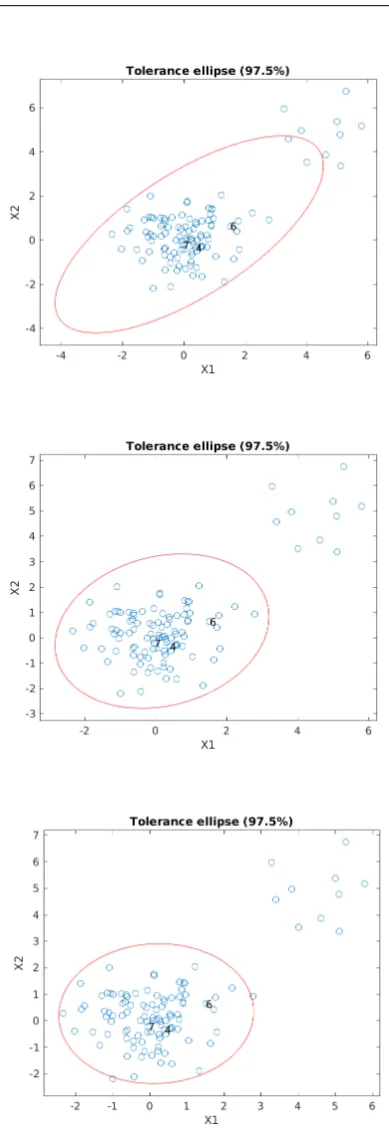
Then from tables 1 to 18, we can clearly see that the MCD-estimator performs best under progressively worse outliers. Even for R = 30, the average covari-ance matrix did almost not differ from the previous two averages. The sample covariance matrix becomes no longer a valid choice while the ˆC-estimator does not suffer much but permanently starts too high. Fig-ure 3 and those above it show a visual representation of the ellips described by the different estimators for the covariance.

Lastly a very important conclusion must be drawn: from this paper we can conclude that robust esti-mation helps in the facial recognition branch of the biometrics. Whilst the author was unable to im-plement the MCD-estimator for the LDA-classifier test, the implementation of the ˆC-estimator shows immediately a positive result. The author however is aware that in practical cases, the test is ran multiple times for many pairs of faces, same class or not. He recommends starting here for future testing of robust estimates.

8 Acknowledgement

The author would like to think dr. ir. L.J. Spreeuwers for his supervision and help. He would also like to thank dr. ir. J. Goseling for his role as the external supervisor. Then a special thanks to the reviewing bachelor committee consisting of the two aforemented

[image:10.595.315.510.82.656.2]

(11)

References

[1] I. van der Ploeg, “Genetics, biometrics and the informatization of the body,”ANNALI-ISTITUTO SUPERIORE DI SANITA, vol. 43, no. 1, p. 44, 2007.

[2] L. Spreeuwers, “Fast and accurate 3d face recognition,”International journal of computer vision, vol. 93, no. 3, pp. 389–414, 2011.

[3] L. Spreeuwers, “Breaking the 99% barrier: optimisation of three-dimensional face recognition,”IET biometrics, vol. 4, no. 3, pp. 169–178, 2015.

[4] D. Pe˜na and F. J. Prieto, “Multivariate outlier detection and robust covariance matrix estimation,”

Technometrics, vol. 43, no. 3, pp. 286–310, 2001.

[5] F. R. Hampel, “Contribution to the theory of robust estimation,”Ph. D. Thesis, University of California, Berkeley, 1968.

[6] R. Gnanadesikan and J. R. Kettenring, “Robust estimates, residuals, and outlier detection with multiresponse data,”Biometrics, pp. 81–124, 1972.

[7] R. A. Maronna and V. J. Yohai, “Robust estimation of multivariate location and scatter,”Wiley StatsRef: Statistics Reference Online, 1976.

[8] M. Hubert and M. Debruyne, “Minimum covariance determinant,”Wiley interdisciplinary reviews: Computational statistics, vol. 2, no. 1, pp. 36–43, 2010.

[9] D. Donoho, I. Johnstone, P. Rousseeuw, and W. Stahel, “Discussion: projection pursuit,”The Annals of Statistics, vol. 13, no. 2, pp. 496–500, 1985.

[10] S. Van Aelst and P. Rousseeuw, “Minimum volume ellipsoid,”Wiley Interdisciplinary Reviews: Computational Statistics, vol. 1, no. 1, pp. 71–82, 2009.

[11] F. Hampel, E. Ronchetti, P. Rousseeuw, and W. Stahel, “Robust statistics, j,”Wiley& Sons, New York, 1986. [12] G. J. McLachlan, “Mahalanobis distance,” Resonance, vol. 4, no. 6, pp. 20–26, 1999.

[13] C. Croux and G. Haesbroeck, “Influence function and efficiency of the minimum covariance determinant scatter matrix estimator,”Journal of Multivariate Analysis, vol. 71, no. 2, pp. 161–190, 1999.

[14] R. Couillet, F. Pascal, and J. W. Silverstein, “Robust estimates of covariance matrices in the large dimensional regime,”IEEE Transactions on Information Theory, vol. 60, no. 11, pp. 7269–7278, 2014.

[15] P. J. Rousseeuw and K. V. Driessen, “A fast algorithm for the minimum covariance determinant estimator,”

Technometrics, vol. 41, no. 3, pp. 212–223, 1999. [16] P. J. Huber,Robust statistical procedures. SIAM, 1996.

[17] G. T. Gilbert, “Positive definite matrices and sylvester’s criterion,”The American Mathematical Monthly, vol. 98, no. 1, pp. 44–46, 1991.

[18] J. J. Sylvester, “Xxxvii. on the relation between the minor determinants of linearly equivalent quadratic functions,”Philosophical Magazine Series 4, vol. 1, no. 4, pp. 295–305, 1851.

[19] P. J. Rousseeuw and C. Croux, “Alternatives to the median absolute deviation,”Journal of the American Statistical association, vol. 88, no. 424, pp. 1273–1283, 1993.

[20] A. M. Pires and J. A. Branco, “Partial influence functions,” Journal of Multivariate Analysis, vol. 83, no. 2, pp. 451–468, 2002.

[21] K. Long, “Gateaux differentials and frechet derivatives.” http://www.math.ttu.edu/ klong/5311-spr09/diff.pdf. [22] P. Zegers, “Fisher information properties,”Entropy, vol. 17, no. 7, pp. 4918–4939, 2015.

[23] J. S. Golan, “Moore–penrose pseudoinverses,”The Linear Algebra a Beginning Graduate Student Ought to Know, pp. 441–452, 2012.

[24] B. D. Ripley,Modern applied statistics with S. Springer, 2002.