Mobile Price Class prediction using Machine Learning Techniques

Mobile Price Class prediction using Machine Learning

Techniques

Muhammad Asim

UET Lahore Pakistan

Zafar Khan

UET Lahore Pakistan

ABSTRACT

To predict “If the mobile with given features will be Economical or Expensive” is the main motive of this research work. Real Dataset is collected from website www.GSMArena.com . Different feature selection algorithms are used to identify and remove less important and redundant features and have minimum computational complexity. Different classifiers are used to achieve as higher accuracy as possible. Results are compared in terms of highest accuracy achieved and minimum features selected. Conclusion is made on the base of best feature selection algorithm and best classifier for the given dataset. This work can be used in any type of marketing and business to find optimal product(with minimum cost and maximum features). Future work is suggested to extend this research and find more sophisticated solution to the given problem and more accurate tool for price estimation.

General Terms

Machine Learning

Keywords

Machine Learning, Prediction, Decision Tree, Naïve Bayes

1.

INTRODUCTION

Price is the most effective attribute of marketing and business. The very first question of costumer is about the price of items. All the costumers are first worried and thinks “If he would be able to purchase something with given specifications or not”. So to estimate price at home is the basic purpose of the work. This paper is only the first step toward the above mentioned destination.

Artificial Intelligence-which makes machine capable to answer the questions intelligently- now a days is very vast engineering field. Machine learning provides us best techniques for artificial intelligence like classification, regression, supervised learning and unsupervised learning and many more. Different tools are available for machine learning tasks like MATLAB, Python, cygwin, WEKA etc. We can use any of classifiers like Decision tree , Naïve Bayes and many more. Different type of feature selection algorithms are available to select only best features and minimize dataset. This will reduce computational complexity of the problem. As this is optimization problem so many optimization techniques are also used to reduce dimensionality of the dataset.

Mobile now a days is one of the most selling and purchasing device. Every day new mobiles with new version and more features are launched. Hundreds and thousands of mobile are sold and purchased on daily basis. So here the mobile price_class prediction is a case study for the given type of problem i.e finding optimal product. The same work can be done to estimate real price of all products like cars, bikes , generators, motors, food items, medicine etc.

Many features are very important to be considered to estimate price of mobile. For example Processor of the mobile. Battery timing is also very important in todays busy schedule of human being. Size and thickness of the mobile are also important decision factors. Internal memory, Camera pixels, and video quality must be under consideration. Internet browsing is also one of the most important constraints in this technological era of 21st century. And so is the list of many features based upon those, mobile price is decided. So we will use many of above mentioned features to classify whether the mobile would be very_economical, economical, expensive or very_ expensive.

The structure of the paper is as follows. Next section is review of previous work.3rd Section contains Methodology and Experimental procedure. Section 4 is the summary of the results. Comparative study is done in section 5. After that paper is concluded in section 6. Outcomes of the work are discussed in section 7. At last in 8th section some suggestions about future work are given.

2.

PREVIOUS WORK

Using previous data to predict price of available and new launching product is an interesting research background for machine learning researchers. Sameerchand-Pudaruth [1] predict the prices of second hand cars in Mauritius. He implemented many techniques like Multiple linear regression, k-nearest neighbors(KNN), Decision Tree, and Naïve Bayes to predict the prices. Sameerchand-Pudaruth got Comparable results from all these techniques. During research it was found that most popular algorithms i.e Decision Tree and Naïve Bayes are unable to handle, classify and predict Numerical values. Number of instances for his research was only 97(47 Toyota+38 Nissan+12 Honda). Due to less number of instances used, very poor prediction accuracies were recorded[1].

Shonda Kuiper[2] has also worked in the same field. Kuiper used multivariate regression model to predict price of 2005 General Motor cars. He collected the data from available online source www.pakwheels.com. The main part of this research work is “Introduction of suitable variable selection techniques, which helped to find that which variables are more suitable and relevant for inclusion in model. This (His research) helps students and future researchers in many fields to understand the conditions under which studies should be conducted and gives them the knowledge to discern when appropriate techniques should be used[2].

handles high dimensional data better and avoids both the under-fitting and over-fitting issues. To find important features for SVM Listiani used Genetic Algorithm . However, the technique failed to show in terms of variance and mean standard deviation why SVM is better than simple multiple regression[3].

Neural Networks (NN) are more better in estimating price of house, this was concluded in the research of Limsombunchai[4]. By comparing with hedonic method his method was more accurate.Operation of both the methods are same, but in NN the model is trained first and then tested for prediction. Using both the methods NN produced higher R-sq and smaller root mean square error (RMSE), while hedonic produced lower values. This research was limited because the actual house price were missing and only estimated prices were used for the research work[4].

K Noor and Saddaqat J [5] also worked to predict the price of Vehicles using different techniques. The researchers achieved highest accuracy using multiple linear regression. This paper proposes a system where price is dependent variable which is predicted, and this price is derived from factors like vehicle’s model, make, city, version, color, mileage, alloy rims and power steering[5].

3.

METHODOLOGY

The experiment is performed using WEKA (Waikato Environment for Knowledge Analysis). The main steps of machine learning are as follows

3.1

Data Collection

Ten features of mobiles are collected from www.GSMArena.com[6] i.e

Catagory( whether the given mobile is made by Apple, Samsung, Lenovo, NOKIA etc). Memory card slot is considered as feature whether it is present or not.

Size of display(Inches), weight(g), Thickness(mm), Internal memory size(GB), Camera Pixels(MP), Video Quality ,

[image:2.595.317.552.136.226.2]

RAM size(GB) and Battery (mAh) , all these attributes have real values with following distinctions.

Table 1. Dataset distinct values

Features Minimum Maximum Mean StdDiv

Display size(inches)

2.8 12.9 6.0 1.7

Weight(gm) 100.0 677.0 205.9 110.7

Thickness(mm) 6.0 12.8 8.2 1.1

Internal memory(GB)

0.5 256.0 39.4 33.2

Features Minimum Maximum Mean StdDiv

Camera(MP) 2.0 23.0 12.7 5.4

Video quality 240.0 2160.0 1437.7 571.1

RAM(GB) 0.5 6.0 2.9 1.4

Battery(mAh) 300.0 8827.0 3366.4 1481.7

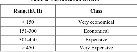
[image:2.595.58.280.378.450.2]

Class is Price_class to predict whether the mobile is Very_economical, Economical, Expensive or Very_Expensive. Basically price is also a continuously changing real value, but it is mapped into above four classes with following criteria.

Table 2. Classification criteria

So a regression problem is converted into classification. Because the main weakness of decision trees and naive bayes classifier is their inability to handle output classes with numeric values. Hence, the price attribute had to be classified into classes which contained a range of prices but this evidently introduced further grounds for inaccuracies[1]. To evaluate the classifier performance data is divided into Training set and test set , 108 instances for training and 28 instances for test set (total 134 instances).

3.2

Dimensionality Reduction

Dimensionality reduction is the process of reducing the number of random variables(Features) under consideration, by obtaining a set of principal variables[7]. The higher the number of features, the harder it gets to visualize the training set and then work on it. Sometimes, most of these features are correlated, and hence redundant. This is where dimensionality reduction algorithms come into play[7].

Two types of Dimensionality reduction algorithms are there ie Feature selection, Feature extraction.

3.2.1

Feature Selection

In feature selection we are interested in finding k of the d dimensions that give us the most information, and we discard the other (d − k) dimensions[8].

3.2.2

Feature Extraction

In feature extraction we are interested in finding a new set of k dimensions that are combinations of the original d dimensions for example Principal Component Analysis[8] .

Here feature selection algorithms are used. There are two approaches: Forward selection and backward selection.

3.2.1.1 Forward Selection

In forward selection, we start with no variables and add them one by one, at each step adding the one that decreases the error the most, until any further addition does not decrease the error (or decreases it only slightly).

3.2.1.2 Backward Selection

In backward selection we start with all variables and remove them one by one, at each step removing the one that decreases the error the most (or increases it only slightly), until any further removal increases the error significantly[8].

Two feature selection algorithm are used InfoGainEval and

WrapperattributEval. InfoGainAttributeEval evaluates the worth of an attribute by measuring the information gain with respect to the class[9]. It gives us Ranked list from maximum

Data Collection

Dimesionality

Reduction Classification

Range(EUR) Class

< 150 Very economical

151-300 Economical

301-450 Expensive

important feature to minimum important features. While WrapperattributEval where the process of feature extraction is thought to “wrap” around the learner it uses as a subroutine[8]. It gives us only list of important feature.

3.2.1.3 InfoGainAttributeEval Algorithm

It gives us the following ranked list of attributes.

Fig 1:Attributes Ranked list by InfoGainAttributeEval algorithm

[image:3.595.315.543.68.337.2]

Figure 1 is screen shot of Ranked list with respect to importance got from InfoGainAttributeEval algorithm. So attributes will be removed in the following pattern.

Table 3. Removing of attributes one by one

Table 3 shows the feature removing process for backward selection. First it is classified with all 10 features, then removed Battery least important one, then weight, then card slot, then Display and then Thickness. Accuracy rate is noted at each stage.

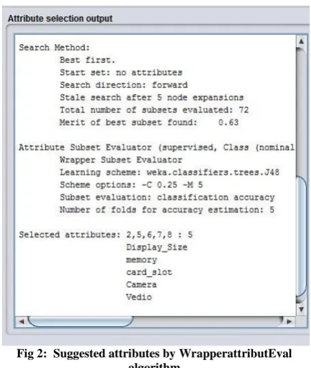
3.2.1.4 WrapperattributEval

It gives us the following list of only important attributes.

Fig 2: Suggested attributes by WrapperattributEval algorithm

Figure 2 is screen shot of the selected attributes by using of WrapperattributEval algorithm, so attributes will be added in the following pattern.

Table 4. Addition of attributes

Table 4 shows the feature Addition process for Forward selection. First classification is done with only one feature Display size, then added Memory, then card slot, then camera, and then Video. Accuracy rate is noted at each stage.

3.3

Classification

Now let’s go through last step that’s classification. As mentioned above separate test set is used to evaluate classifier and find accuracy. Any classification is correct if it can be judged by calculating the number of correctly identified class samples (true positives), the number of correctly identified samples that are not members of the class (true negatives) and samples that either were incorrectly allocated to the class (false positives) or that were not identified as class samples (false negatives)[10]. Accuracy tells us percentage of correctly classified instances. Mathematically

100

*

_

_

_

Samples

Total

Samples

Classified

Correctly

Accuracy



Classifier is trained by training set. Two classifiers are used i.e Decision Tree (J48) classifier and Naive Bayes classifier. Classifier output for first classification is shown below.

Removal of Attributes

No attribute removed Battery Weight Card slot

Display Thickness

RAM

Addition Of Attributes

Display Size Memory Card slot Camera

[image:3.595.53.283.135.378.2] [image:3.595.372.495.392.469.2] [image:3.595.89.224.452.582.2]

[image:4.595.62.282.71.358.2]

Fig 3: 1st _{Classification Results}

Decision tree classifier output is shown. Time taken by this classifier is 0.02 seconds to build the model and 0.01sec to test it. Twenty instances are classified correctly out of 28 with 71.42% accuracy rate. Please note that it is first classification where all 10 features are used.

4.

RESULTS SUMMARY

Now to summarize the work, all the results and their graphs are presented for comparative study.

4.1

Results of InfoGainAttributeEval

Algorithm and Decision Tree Classifier

Table 5. Accuracy and number of attributes

Graph 1. Accuracy vs number of attributes

Maximum accuracy achieved in this specific combination is 75 %, and features selected are 5, above 5 features are discarded. When RAM is added accuracy started decreasing because it is redundant or irrelevant data for this specific combination of classifier and feature selection algorithm.

4.2

Results of InfoGainAttributeEval

algorithm and Naive Bayes Classifier

Table 6. Accuracy and number of attributes

Graph 2. Accuracy vs number of attributes

Maximum accuracy achieved in this specific combination is 71.42 %, and features selected are 6 above 4 features are discarded. When Thickness is added accuracy started

60 65 70 75 80

10 9 8 7 6 5

A

cc

u

rac

y

%

Attributes

InfoGainAttributeEval, Decision Tree

55 60 65 70 75

10 9 8 7 6

A

cc

u

ra

cy

%

Attributes

InfoGainAttributeEval, Naive Bayes InfoGainAttributeEval , Decision Tree

# of Attributes

Accuracy %

Removal of Attributes

10 71.428 No

9 71.42 Battery

8 71.42 Weight

7 71.42 Card slot

6 75 Display

5 75 Thickness

4 57.14 RAM

InfoGainAttributeEval, Naive Bayes

# of Attributes Accuracy (%) Removal of Attributes

10 60.7 No

9 60.7 Battery

8 67.857 Weight

7 71.42 Card slot

6 71.42 Display

[image:4.595.312.544.72.247.2]

decreasing because it is redundant or irrelevant data for this specific combination of classifier and feature selection algorithm.

4.3

Results of WrapperattributEval

algorithm and Decision Tree Classifier

Table 7. Accuracy and number of attributes

Graph 3. Accuracy vs number of attributes

Maximum accuracy achieved in this specific combination is 78 %, and features selected are 2. All except these two features are discarded. When card slot and other features is added accuracy started decreasing because it is redundant or irrelevant data for this specific combination of classifier and feature selection algorithm.

4.4

Results of WrapperattributEval

algorithm and Naïve Bayes Classifier

Table 8. Accuracy and number of attributes

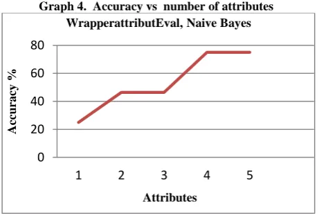
Graph 4. Accuracy vs number of attributes

Maximum accuracy achieved in this specific combination is 75 %, and features selected are 5. All except these five features are discarded. When other features is added accuracy started decreasing because of redundancy or irrelevancy of data for this specific combination of classifier and feature selection algorithm.

5.

COMPARATIVE STUDY

[image:5.595.315.546.73.228.2]

Comparison in machine learning is done in terms of Maximum accuracy and minimum number of features selected. Maximum accuracy means more data classified correctly. While minimum number of feature means minimum memory required and reduced computation complexity.

Table 9. Comparative Study

Comparing the results maximum accuracy achieved is 78%, when WrapperattributEval algorithm is used for feature selection and Decision tree as a classifier. The features selected are only best two features (Display size and memory in GB) out of ten. So the given is best combination for the given specific data.

6.

CONCLUSION

This work can be concluded with the comparable results of both Feature selection algorithms and classifier except the combination of WrapperattributEval and Descision Tree J48 classifier. This combination has achieved maximum accuracy and selected minimum but most appropriate features. It is important to note that in Forward selection by adding irrelevant or redundant features to the data set decreases the efficiency of both classifiers. While in backward selection if we remove any important feature from the data set, its efficiency decreases. The main reason of low accuracy rate is low number of instances in the data set. One more thing should also be considered while working that converting a regression problem into classification problem introduces more error.

30 40 50 60 70 80 90

1 2 3 4 5

Ac

cu

ra

cy

%

Attributes

WrapperattributEval, Decision Tree

0 20 40 60 80

1 2 3 4 5

Ac

cu

ra

cy

%

Attributes

WrapperattributEval, Naive Bayes

WrapperattributEval , Decision Tree

# of Attributes

Accuracy %

Addition Of Attributes

1 39.28 Display Size

2 78 Memory

3 67.85 Card slot

4 71.42 Camera

5 67.85 video

WrapperattributEval, Naive Bayes # of

Attributes

Accuracy % Addition Of Attributes

1 25 Display Size

2 46.4 Memory

3 46.4 Card slot

4 75 Camera

5 75 Video

# of Selected Features

Accuracy (%)

InfoGa inAttri buteEv

al

Wrappe rattribut Eval

InfoGain Attribut eEval

Wrapp erattri butEva

l

J48 5 2 75 78

Naive Bayes

[image:5.595.315.552.394.528.2]

7.

OUTCOMES OF THE WORK

7.1 Cost prediction is the very important factor of marketing and business. To predict the cost same procedure can be performed for all types of products for example Cars, Foods, Medicine, Laptops etc.

7.2 Best marketing strategy is to find optimal product (with minimum cost and maximum specifications). So products can be compared in terms of their specifications, cost, manufacturing company etc.

7.3 By specifying economic range a good product can be suggested to a costumer.

8.

FUTURE WORK EXTENSION

8.1

More sophisticated artificial intelligence techniques can be used to maximized the accuracy and predict the accurate price of the products.

8.2

Software or Mobile app can be developed that will predict the market price of any new launched product.

8.3

To achieve maximum accuracy and predict more accurate, more and more instances should be added to the data set. And selecting more appropriate features can also increase the accuracy. So data set should be large and more appropriate features should be selected to achieve higher accuracy.

9.

REFERENCES

[1] Sameerchand Pudaruth . “Predicting the Price of Used Cars using Machine Learning Techniques”, International Journal of Information & Computation Technology. ISSN 0974-2239 Volume 4, Number 7 (2014), pp. 753-764

[2] Shonda Kuiper, “Introduction to Multiple Regression: How Much Is Your Car Worth? ” , Journal of Statistics Education · November 2008

[3] Mariana Listiani , 2009. “Support Vector Regression Analysis for Price Prediction in a Car Leasing Application”. Master Thesis. Hamburg University of Technology.

[4] Limsombunchai, V. 2004. “House Price Prediction: Hedonic Price Model vs. Artificial Neural Network”, New Zealand Agricultural and Resource Economics Society Conference, New Zealand, pp. 25-26. 2004 [5] Kanwal Noor and Sadaqat Jan, “Vehicle Price Prediction

System using Machine Learning Techniques” , International Journal of Computer Applications (0975 – 8887) Volume 167 – No.9, June 2017.

[6] Mobile data and specifications online available from https://www.gsmarena.com/ (Last Accessed on Friday, ‎December ‎22, ‎2017, ‏‎6:14:54 PM)

[7] Introduction to dimensionality reduction, A computer

science portal for Geeks.

https://www.geeksforgeeks.org/dimensionality-reduction/ (Last Accessed on Monday , Jan 2018 22, 3 PM)

[8] Ethem Alpaydın, 2004. Introduction to Machine Learning, Third Edition. The MIT Press Cambridge, Massachusetts London, England

[9] InfoGainAttributeEval-Weka Online available from http://weka.WrapperattributEval/doc.dev/weka/attributeS election/InfoGainAttributeEval.html (Last Accessed in Jan 2018 )