Accuracy Assessment of Land Use/Land Cover Classification Using Remote Sensing and GIS

ISSN Online: 2156-8367 ISSN Print: 2156-8359

Accuracy Assessment of Land Use/Land Cover

Classification Using Remote Sensing and GIS

Sophia S. Rwanga

, J. M. Ndambuki

1_{Department of Civil Engineering, Tshwane University Technology, Pretoria, South Africa} 2_{Department of Civil Engineering, Vaal University of Technology, Vanderbijlpark, South Africa} 3_{Department of Civil Engineering, Tshwane University of Technology, Pretoria, South Africa}

Abstract

Remote sensing is one of the tool which is very important for the production of Land use and land cover maps through a process called image classification. For the image classification process to be successfully, several factors should be considered including availability of quality Landsat imagery and secondary data, a precise classification process and user’s experiences and expertise of the procedures. The objective of this research was to classify and map land-use/land-cover of the study area using remote sensing and Geospatial Information System (GIS) techniques. This research includes two sections (1) Landuse/Landcover (LULC) classification and (2) accuracy assessment. In this study supervised classification was performed using Non Parametric Rule. The major LULC classified were agriculture (65.0%), water body (4.0%), and built up areas (18.3%), mixed forest (5.2%), shrubs (7.0%), and Barren/bare land (0.5%). The study had an overall classification accuracy of 81.7% and kappa coefficient (K) of 0.722. The kappa coefficient is rated as substantial and hence the classified image found to be fit for further research. This study present essential source of information whereby planners and decision makers can use to sustainably plan the environment.

Keywords

Accuracy assessment, Geographic Information Systems (GIS), Land Use Land Cover (LULC), Remote Sensing

1. Introduction

Land use and land cover information is required for policy making, business and administrative purposes. With their spatial details, the data are likewise crucial for environmental protection and spatial planning. Landuse classification is vital

How to cite this paper: Rwanga, S.S. and Ndambuki, J.M. (2017) Accuracy Assess-ment of Land Use/Land Cover Classifica-tion Using Remote Sensing and GIS. Inter-national Journal of Geosciences, 8, 611-622. https://doi.org/10.4236/ijg.2017.84033

Received: February 14, 2017 Accepted: April 27, 2017 Published: April 30, 2017

Copyright © 2017 by authors and Scientific Research Publishing Inc. This work is licensed under the Creative Commons Attribution International License (CC BY 4.0).

S. S. Rwanga, J. M. Ndambuki

because it gives data which can be used as input for modeling, especially the one dealing with environment, for instance models deals with climate change and policies developments [1]. Hence the combined LULC grant a comprehensive means of understanding the interaction of geo-biophysical, socioeconomic sys-tems behaviors and interactions [2]. To provide more useful information in land cover, Remote Sensing is often paired with Geographic Information System (GIS) technique.

Remote sensing is the main source for several kinds of thematic data critical to GIS analyses, including data on landuse and landcover characteristics. Aerial and Landsat satellite images are also frequently used to evaluate land cover distribu-tion and to update existing geospatial features. With the introducdistribu-tion of remote sensing systems and image processing software, the importance of remote sens-ing in Geospatial Information System (GIS) has expanded significantly [3]. The accelerated usage of remote sensing data and techniques has made geospatial process faster and powerful, although the increased complexity also creates in-creased possibilities for error [4]. Previously, accuracy assessment was not a priority in image classification studies. However, because of the accelerated chances for error presented by digital imagery, accuracy assessment has become a very vital process [5].

Accuracy assessment or validation is a significant step in the processing of remote sensing data. It establishes the information value of the resulting data to a user. Productive utilization of geodata is only possible if the quality of the data is known. The overall accuracy of the classified image compares how each of the pixels is classified versus the definite land cover conditions obtained from their corresponding ground truth data. Producer’s accuracy measures errors of omis-sion, which is a measure of how well real-world land cover types can be classi-fied. User’s accuracy measures errors of commission, which represents the like-lihood of a classified pixel matching the land cover type of its corresponding real-world location [5][6][7]. The error matrix and kappa coefficient have be-come a standard means of assessment of image classification accuracy. Moreo-ver, Error matrix have been used in numerous land classification studies and were a crucial component of this research.

The objective of this research was to classify and map land-use/land-cover of the study area using remote sensing and Geospatial Information System (GIS) techniques and to carry out accuracy assessment in order to find out how well the classification procedures was undertaken and also to understand how to in-terpret the usefulness of the classification.

Study Area

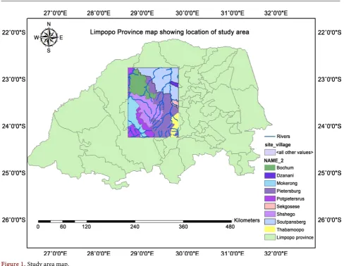
The study area map was prepared from Limpopo province map. The area falls under latitude 23˚0'31.0956"S, 29˚30'48.5697"E and longitude 24˚2'48.3007"S and

29˚32'16.9088"E. The total study area is 7138 km2. The rainfall (average) ranges

Figure 1. Study area map.

2. Materials and Methods

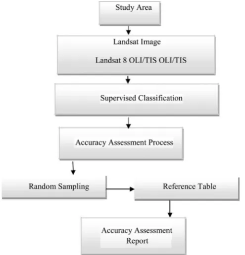
This paper covers two sections: 1) Landuse/Landcover (LULC) classification and 2) accuracy assessment. The landuse/cover classification of the study area and accuracy assessment were carried out as per the methodology presented in

Fig-ure 2.

Landuse/Landcover Classification

Classification process and analysis of the different LULC classes were done using two Landsat satellite images covering the Landsat 8 OLI/TIS acquired on 16 September 2015. These images includes; L8 OLI/TIRS (path 170, rows 68) and L8 OLI/TIRS (path 170, rows 77) (Table 1). The Landsat images were down-loaded from United States Geological (USGS) Earth Explorer

(https://earthexplorer.usgs.gov/). The selection of the Landsat satellite images dates was influenced by the quality of the image especially for those with limited or low cloud cover. Each Landsat was georeferenced to the WGS_84 datum and Universal Transverse Mercator Zone 35 North coordinate system.

S. S. Rwanga, J. M. Ndambuki

Figure 2. Schematic of work flow for LULC and accuracy assessment.

Table 1. Details of Landsat 8 OLI/TIS used for classification.

Satellite Sensor _ID Path/row Layers Date of acquisition Grid cell _{size (m)}

Landsat 8 OLI/TIS LC81700762015259LGN00 _{LC81700762015259LGN00} 170/77 _170/68 11 16 September 2015 30

stacking were carried out in order to Ortho-rectify the satellite images. The im-age was then processed in ERDAS IMAGINE 2015 software. The satellite imim-age of each band was stacked in ERDAS Hexagon within interpreter main icon utili-ties with layer stacked function. Then, from the stacked satellite image the study area image was extracted by clipping the study area using ArcGIS 10.3 software.

Landuse/Landcover (LULC) Classification: Supervised

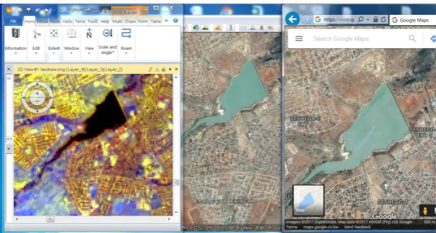
For this study, only supervised classification was performed. Supervised classifi-cation according to [8] is where “the user develops the spectral signatures of known categories, such as urban and forest, and then the software assigns each pixel in the image to the cover type to which its signature is most comparable”. “Supervised classification is the process most frequently used for quantitative analyses of remote sensing image data” [9]. The supervised classification was ap-plied after defined area of interest (AOI) which is called training classes. More than one training area was used to represent a particular class. The training sites were selected in agreement with the Landsat Image, Google Earth and Google Map (Figure 3). The basic sequence operation followed on supervised classifica-tion was;

classifi-cation is to define the areas that will be used as training sites for each land cover class. This is usually done by using the on-screen digitized features. The created features are called Area of Interest (AOI).The selection of the training sites was based on those areas clearly identified in all sources of im-ages. In this study, one hundreds training sites were been identified.

• _{Extraction of Signatures: After the training site (AOI) being digitized, the}

next step was to create statistical characterizations of each information. These are called Signatures editors in ERDAS Imagine 2015. In this step, the goal was to create a signal (SIG) file for every informational class. The SIG files contain a variety of information about the land cover classes described. After the entire signature have been created, then the SIG file saved as dialog

(Table 2).

• _{Classification of the Image (Supervised classification): The supervised}

classi-fication has been applied after defined training classes. One or more than one training area was used to represent a particular class. During the supervised classification process, the entire Signature editor was selected in order to be used on the classification process. Then the classify was selected from the

Figure 3. Identification of training sites using Landsat image (Erdas Imagine 2015), Google earth and Google map.

Table 2. Signature editor table for classified image.

Class # Signature name Color Red Green Blue Value Order Count Prob. 1 Mixed forest 0.000 0.392 0.000 8 166 1267 1.000 2 Barren/bare land 0.824 0.706 0.549 3 168 87 1.000

3 Shrubs 0.101 0.899 0.730 6 169 50 1.000

S. S. Rwanga, J. M. Ndambuki

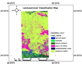
Figure 4. Classified map of study area.

Table 3. Landcover classification scheme.

Land cover Description

Water body Lakes, reservoirs, stream, rivers, swamps

Built up areas Land covered by buildings and other man-made structures. Residential, _{commercial services, industrial area, mixed urban or built up lands}

Barren/bare land

Lands with exposed soil, sand or rocks, and never has more than 10% vegetated cover during any time of the year. Bare ground, bare exposed rocks, strip mines, quarries and gravel pits

Shrubs Lands with woody vegetation less than 2 meters tall. The shrub foliage can be _{either evergreen or deciduous}

Mixed forest Lands dominated by trees with a percent cover >60% and height exceeding 2 _{meters, Deciduous forest land and evergreen forest land}

Agriculture Lands covered with temporary crops followed by harvest period, Crop fields and _pastures

Editor Menu bar, classify/supervised. Non Parametric Rule was used in this classification. The Image was classified into six classes namely; Waterbody, Built up areas, Barren/bare land, shrubs, Mixed forest and Agriculture (Table 3).

Classification Results and Discussion

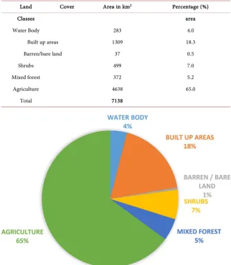
(0.5%) (See Figure 5). Agriculture was found to be the dominant type of Land use classified which covers about 65.0% of the total study area, followed by Built-up areas while the least classified was Barren/bare land which accounts for 0.5%. During the classification, among the water body classified were rivers (sand river and Houtriver).

3. Classification Accuracy Assessment

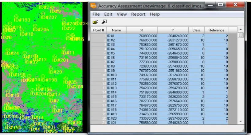
One of the most important final step at classification process is accuracy assess-ment. The aim of accuracy assessment is to quantitatively assess how effectively the pixels were sampled into the correct land cover classes. Moreover the key emphasis for accuracy assessment pixel selection was on areas that could be clearly identified on both Landsat high resolution image, Google earth and Google Map. A total of 307 points (locations) were created in the classified im-age of the study area. The Accuracy Assessment Cell Array Reference column was filled according to the best guess of each reference point. Hydrogeological

Table 4. Classified area under different Landuse classes in study area.

Land Cover Area in km2 _{Percentage (%)}

Classes area

Water Body 283 4.0

Built up areas 1309 18.3

Barren/bare land 37 0.5

Shrubs 499 7.0

Mixed forest 372 5.2

Agriculture 4638 65.0

Total 7138

S. S. Rwanga, J. M. Ndambuki

Figure 6. Landsat (classified) image of the study area covered with 307 points from random sampling.

Table 5. Theoretical error matrix of LULC classification.

S. No Classified Water _body Built up _areas Barren/bare _land Shrubs Mixed _{forest Agriculture Total Correct sampled}

1 Water body 20 3 3 0 0 1 27 20

2 Built up areas 2 61 23 1 3 2 92 61

3 Barren/bare land 0 0 12 0 0 0 12 12

4 Shrubs 0 2 4 25 0 3 34 25

5 Mixed forest 0 0 3 2 31 1 37 31

6 Agriculture 1 1 0 0 1 102 105 102

Total 23 67 45 28 35 109 307 251

map series of the republic of South Africa, Topographic map, Google earth and Google Map were used as reference source to classify the selected points.

Table 5 shows the relationship between ground truth data and the

corres-ponding classified data obtained through error matrix report.

The overall classification accuracy = No. of correct points/total number of points 251 81.7%

307

= = _.

Table 5 shows a theoretical confusion matrix (error matrix) of a LULC

classi-fication. The columns of the confusion matrix show to which classes the pixels is in the validation set belong (ground truth) and the rows show to which classes the image pixels have been assigned to in the image. The diagonal show the pix-els that are classified correctly. Pixpix-els that are not assigned to the proper class do not occur in the diagonal and give an indication of the confusion between the different land-cover classes in the class assignment.

corres-ponding to the row, represent the commission errors and describe the confusion between that image class and describes the other land-cover classes. The com-mission errors describe the chance that a pixel that has been assigned to a par-ticular class actually belongs to one of the other classes.

Moreover, this study considered other metrics derived from the error matrix to further describe accuracy assessments including; commission and omission error, sensitivity and specificity, positive and negative predictive power and Kappa statistics. For thorough information of these concepts, refer to [10] and

[11].

In this research, various statistics related with classification accuracy as well as overall Kappa statistic are computed based on [12] formulation as indicated be-low:

(

)

(

)

Sensitivity equivalent to Producer s Accuracy

Specificity

Commision error 1 Specificity

Ommision error 1 Sensitivity

Positive Predictive Power Equivalent to User's accuracy

Negative Predictive ' P a a b d b d a a b = + = + = − = − = + ower d c d = + where:

a = number of times a classification agreed with the observed value

b = number of times a point was classified as X when it was observed to not be X.

c = number of times a point was not classified as X when it was observed to be X.

d = number of times a point was not classified as X when it was not observed to be X. Total points = N = (a + b + c + d)

KAPPA analysis is a discrete multivariate technique used in accuracy assess-ments [13]. KAPPA analysis yields a Khat statistic (an estimate of KAPPA) that is a measure of agreement or accuracy [5]. The Khat statistic is computed as;

(

)

(

)

ii i i

i r

ii i

N x x Xx

K

N x Xx

+ = = + = − + = −

∑

∑

∑

r = number of rows and columns in error matrix, N = total number of

obser-vations (pixels)

Xii= observation in row i and column i,

Xi+ = marginal total of row i, and X+i = marginal total of column i

S. S. Rwanga, J. M. Ndambuki

Table 6. Rating criteria of Kappa statistics.

S.No Kappa statistics Strength of agreement

1 <0.00 Poor

2 0.00 - 0.20 Slight

3 0.21 - 0.40 Fair

4 0.41 - 0.60 Moderate

5 0.61 - 0.80 Substantial

6 0.81 - 1.00 Almost perfect

Table 7. Category wise accuracy assessment statistical parameters.

Observed proportion of

agreements (Po) Expected proportion of agreement (Pe) Kappa coefficient (K)

0.9674 0.850 0.782

0.8795 0.613 0.689

0.8632 0.805 0.298

0.9609 0.818 0.785

0.9674 0.793 0.843

0.9707 0.547 0.935

Table 8. Category wise accuracy assessment statistical parameters.

Classified Data Parameters

Sensitivity Specificity Commission Error Omission Error UA PA Water body 0.8696 0.97535 0.0246 0.1304 0.741 0.870 Built up areas 0.9104 0.87083 0.1292 0.0896 0.663 0.910

Barren/bare

land 0.2667 0.96565 0.0344 0.7333 0.571 0.267 Shrubs 0.8929 0.96774 0.0323 0.1071 0.735 0.893 Mixed forest 0.8857 0.97794 0.0221 0.1143 0.838 0.886 Agriculture 0.9444 0.98492 0.0151 0.0556 0.971 0.936

Results and Discussion on Accuracy Assessments

Using the formulae furnished on section 3.0, various accuracy evaluating para-meters were computed and tabulated in Table 7 and Table 8.

field. Agriculture was found to be more reliable with 97.1% of user accuracy. The commission error reflects the points which are included in the category while they really do not belong to that category. For instance, the commission error is highest in case of built - up areas which meant that more number of points (31) which do not fall under this category are classified as built up areas. Equally, the omission error reflects the number of points which are not included in the category while they really belong to the category. The omission error in case of Barren/bare land is more (0.7333) with 33 points which actually belong to this category not being categorized in this class. In this study an overall Kappa coefficient of 0.722 was obtained which is rated as substantial. Apart from over-all classification accuracy, the above individualized parameters give a classifier a more detailed description of model performance of the particular class or cate-gory of his field of interest or study.

4. Conclusions

Remote sensing is very important for the production of Land Use / Land Cover maps which can be done through a method called image classification. This me-thod had made huge improvements over the past decades in the following four areas for example; LULC maps production at any scale, improvement and use of advanced classification process such as pre field and sub pixel, classification procedures using knowledge base process and incorporation of auxiliary data into classification procedures; such data includes, digital elevation model (DEM), road, soil, landuse and census data. Moreover classifying landsat image-ries in order to obtain accurate and reliable LULC information still remains a challenge that depend on several factors for example the imageries selected, landscape complexity, image processing techniques and classification process it-self.

The accelerated usage of remote sensing data and techniques has made geos-patial process faster and powerful, although the increased complexity also creates increased possibilities for error. The objective of this paper was to classify and map land use - land cover (LULC) of the study area using Remote Sensing and GIS techniques and also to carry out accuracy assessment in order to assess how well a classification worked.

The supervised classification was performed using Non Parametric Rule. The image was classified into six classes; Agriculture (4638 km2_{), water body (283} km2_{), built up areas (1309 km}2_{), mixed forest (372 km}2_{), shrubs (499 km}2_{), and} Barren/bare land (37 km2_{). Agriculture was the dominant type of Landuse} classi-fied which covers about 65.0% of the total study.

S. S. Rwanga, J. M. Ndambuki

as substantial and hence the classified image found to be fit for further research.

References

[1] Disperati, L., Gonario S. and Virdis, P. (2015) Assessment of Land-Use and Land- Cover Changes from 1965 to 2014 in Tam Giang-Cau Hai Lagoon, Central Viet-nam. Applied Geography, 58, 48-64.

[2] Moran, E. F., Skole, D.L. and Turner, B.L. (2004) The Development of the Interna-tional Land-Use and Land-Cover Change (LUCC) Research Program and Its Links to NASA’s Landcover and Land-Use Change (LCLUC) Initiatives. Kluwer Academ-ic PublAcadem-ication, Netherlands.

[3] Merchant, J.W. and Narumalani, S. (2009) Integrating Remote Sensing and Geo-graphic Information Systems. Papers in Natural Resources, Paper 216.

http://digitalcommons.unl.edu/natrespapers/216

[4] Murty, P.S. and Tiwari, H. (2015) Accuracy Assessment of Land Use Classification —A Case Study of Ken Basin. Journal of Civil Engineering and Architecture Re-search, 2, 1199-1206.

[5] Congalton, R.G. (1991) A Review of Assessing the Accuracy of Classifications of Remotely Sensed Data. Remote Sensing of Environment, 37, 35-46.

https://doi.org/10.1016/0034-4257(91)90048-B

[6] Campbell, J.B. (2007) Introduction to Remote Sensing. 4th Edition, The Guilford Press, New York.

[7] Jensen, J.R. (2005) Introductory Digital Image Processing: A Remote Sensing Pers-pective. 3rd Edition, Pearson Prentice Hall, Upper Saddle River, NJ.

[8] Eastman, J.R. (2003) Guide to GIS and Image Processing 14, 239-247. Clark Univer-sity Manual, USA.

[9] Richards, J. and Jia, X. (2006) Remote Sensing Digital Image Analysis: An Introduc-tion.Springer, Berlin.

[10] Fielding, A.H. and J.F. Bell. (1997) A Review of Methods for the Assessment of Pre-diction Errors in Conservation Presence/Absence Models. Environmental Conser-vation, 24, 38-49. https://doi.org/10.1017/S0376892997000088

[11] Lurz, P.W.W., Rushton, S.P., Wauters, L.A., Bertolino, S., Currado, I., Mazzoglio, P. and Shirley, M.D.F. (2001) Predicting Grey Squirrel Expansion in North Italy: A Spatially Explicit Modeling Approach. Landscape Ecology, 16, 407-420.

https://doi.org/10.1023/A:1017508711713

[12] Jenness, J. and Wynne, J.J. (2007) Kappa Analysis (kappa_stats.avx) Extension for ArcView 3.x. Jenness Enterprises.

http://www.jennessent.com/arcview/kappa_stats.htm

[13] Jensen, J.R. (1996) Introductory Digital Image Processing: A Remote Sensing Pers-pective. 2nd Edition, Prentice Hall, Inc., Upper Saddle River, NJ.

Submit or recommend next manuscript to SCIRP and we will provide best service for you:

Accepting pre-submission inquiries through Email, Facebook, LinkedIn, Twitter, etc. A wide selection of journals (inclusive of 9 subjects, more than 200 journals)

Providing 24-hour high-quality service User-friendly online submission system Fair and swift peer-review system

Efficient typesetting and proofreading procedure

Display of the result of downloads and visits, as well as the number of cited articles Maximum dissemination of your research work

Submit your manuscript at: http://papersubmission.scirp.org/