Original citation:
Paterson, Michael S., Pippenger, N. and Zwick, U. (1990) Optimal carry save networks. University of Warwick. Department of Computer Science. (Department of Computer Science Research Report). (Unpublished) CS-RR-166
Permanent WRAP url:
http://wrap.warwick.ac.uk/60861
Copyright and reuse:
The Warwick Research Archive Portal (WRAP) makes this work by researchers of the University of Warwick available open access under the following conditions. Copyright © and all moral rights to the version of the paper presented here belong to the individual author(s) and/or other copyright owners. To the extent reasonable and practicable the material made available in WRAP has been checked for eligibility before being made available.
Copies of full items can be used for personal research or study, educational, or not-for-profit purposes without prior permission or charge. Provided that the authors, title and full bibliographic details are credited, a hyperlink and/or URL is given for the original metadata page and the content is not changed in any way.
A note on versions:
Research report 166
OPTIMAL CARRY SAVE NETWORKS
M S PATERSON, N PIPPENGER, U ZWICK
(RR166)
A general theory is developed for constructing the asymptotically shallowest networks and the asymptotically smallest networks (with respect to formula size) for the carry save addition of n numbers using any given basic carry save adder as a building block.
Using these optimal carry save additional networks the shallowest known multiplication circuits and the shortest formulae for the majority function (and many other symmetric Boolean functions) are obtained.
In this paper, simple basic carry save adders are described using which multiplication circuits of depth 3.71 log
n (the result of which is given as the sum of two numbers) and majority formulae of size 0 (n'•") are constructed. Using more complicated basic carry save adders, not described here, these results could be further improved. Our best bounds are currently 3.57 log n for depth and 0 (n3.13) for formula size.
Optimal Carry Save Networks
Michael S. Paterson *
Nicholas Pippenger t
Uri Zwick
October 8, 1990
Abstract
A general theory is developed for constructing the asymptotically shallowest networks and the asymptotically smallest networks (with respect to formula size) for the carry save addition of n numbers using any given basic carry save adder as a building block.
Using these optimal carry save addition networks the shallowest known multiplication circuits and the shortest formulae for the majority function (and many other symmetric Boolean functions) are obtained.
In this paper, simple basic carry save adders are described using which multiplication circuits of depth 3.71 log n (the result of which is given as the sum of two numbers) and majority formulae of size 0(n3.21) are constructed. Using more complicated basic carry save adders, not described here, these results could be further improved. Our best bounds are currently 3.57 log n for depth and 0(n3.13) for formula size.
1. Introduction
The question 'How fast can we multiply?' is one of the fundamental questions in theoretical computer science. Ofman-Karatsuba [9] and SchOnhage-Strassen [24] (see also [1],[15]) tried to answer it by minimising the number of bit operations required, or equivalently the circuit size. A different approach was pursued by Avizienis [2], Dadda [6], Ofman [17], Wallace [28] and others. They investigated the depth, rather than the size of multiplication circuits.
The main result proved by the above authors in the early 1960's was that, using a process called Carry Save Addition, n numbers (of linear length) could be added in depth O(log n). As a consequence depth O(log n) circuits for multiplication and polynomial
size formulae for all the symmetric Boolean functions are obtained.
*Department of Computer Science, University of Warwick, Coventry, CV4 7AL, England. This author was partially supported by a Senior Fellowship from the SERC and by the ESPRIT II BRA Programme of the EC under contract # 3075 (ALCOM).
tDepartment of Computer Science, University of British Columbia, Vancouver, British Columbia, Canada V6T 1W5. This author was partially supported by an NSERC operating grant and an ASI fellowship award.
They all used a component called a '3 ---+ 2' Carry Save Adder (CSA3_,2) which reduces the sum of three numbers (of arbitrary length) to the sum of only two in a (small) constant depth. It is easy to see that using log3/2 n 0(1) levels of such CSA3_,2's it is possible to reduce the sum of n numbers to the sum of only two. The resulting two numbers could be added (if required) using a Carry Look Ahead Adder (see [3],[10]) with additional depth (1 + o(1)) log m (where m is the length of the numbers).
In this paper we look more carefully at the construction of CSA-networks for carry save addition. A moment's reflection shows that any CSA3_,2-network for the carry save addition of n numbers will have at least log3/2 n levels of CSA3_,2's. Thus, if a CSA3-.2 is regarded as a black box to which the inputs should be supplied simultaneously and which then after a fixed delay returns the two outputs simultaneously, then this naive construction is optimal. It turns out however that, even for the best CSA3_,2's, some of the inputs may be supplied after the others, without delaying the outputs, and that one of the outputs is sometimes produced before the other. The task of constructing networks with minimal total delay in such cases becomes much more interesting.
In general we assume that we are given a CSAk_,I whose delay characteristics are described by a delay matrix M. The entry mi.; of the matrix gives the relative delay of the i-th output with respect to the j-th input. In particular, if the k inputs to a CSAk_,L are ready at times xl, , xk, we assume that the i-th output is ready at
time y, = maxi<j<k{mi; x j }. This corresponds to taking the {max, +} inner product between M and x. We show how to extract from any delay matrix M the minimal constant q such that CSAk,.1-networks for the carry save addition of n numbers with delay (q o(1)) log n can be constructed using CSAk_,t's with delay matrix M. We exhibit explicit constructions achieving this optimal behaviour.
For a given implementation of a CSAk_,I using Boolean circuitry, if we define mi.; to be the length of the longest path from any bit of the j-th input number to any bit of the i-th output number then the above result translates immediately to a result about depth.
Several basic designs of GSA's are described in the next section. Using these designs optimally we get U2-circuits (circuits over the unate dyadic basis U2 = B2 — {®, of depth 5.42 log n and B2-circuits (circuits over the basis B2 of all dyadic Boolean functions) of depth 3.71 log n for the carry save addition of n numbers. Using more complicated GSA's, not described here, these results could be improved to 5.02 log n and 3.57 log n respectively. As a consequence, we derive circuits of depth 6.02 log n and 4.57 log n for the addition of n numbers (of linear length) or for the multiplication of two n bit numbers. This improves a previous result of Khrapchenko [14] and the naive estimates of Ofman and Wallace.
Multiple addition circuits (of n numbers of n bits each) are necessarily of size SZ(n2). Our circuits are composed of 0(n) CSA's each of size 0(n) so they have this optimal size.
depth (cf. [16],[29]). The implied constant factors however are much larger than those obtained here.
Another special case of multiple addition is bit counting. A counter for n bits could be obtained by carry save adding the n input bits, treating each as a number, and then adding the two output numbers. Note that the length of the two output numbers is O(log n) so the additional depth required to add them up in this case is only O(log log n). As a consequence we get depth 5.02 log n U2-circuits and depth 3.57 log n B2-circuits for counting. Many symmetric Boolean functions, such as majority and MODk for any fixed
k, can be computed in depth o(log n) once the bit count is done, so we get the same
bounds for them as well.
An analogous theory is developed for formula size. We assume that the formula size characteristics of a CSAk_,/ are described by an occurrence matrix N. The entry ni; gives the number of appearances of the j-th input number in the formula for the i-th output number. If the k inputs to a CSAk_,/ have formula sizes xl, , xk then the i-th
output number will have formula size yi = nii xi. Note that this corresponds to multiplying the matrix N by the vector x = (x1, . , k).
Again we show how to extract from the occurrence matrix the minimal q such that CSAk_,L-networks of formula size n(9+0(1)) can be constructed and describe constructions with optimal behaviour.
Using the CSA designs of Section 2 optimally we get U2-formulae of size 0(n4-70) and /32-formulae of size 0(723.21) for each output bit in the carry save addition of n numbers and for many symmetric Boolean functions as before. Again, using more complicated GSA's, not described here, these bounds could be improved to 0(124') and 0(n3.13) respectively. These constructions improve previous results of Khrapchenko [13], Pippenger [21], Paterson [18] and Peterson [20].
Depth and the logarithm of formula size are closely connected. It is known for example that log LB2 (1) 5_ DB,(f) _< 2.47 log LB, (f) (in fact even that Du, (f) _< 2.47 log LB2(f))
and that log Lu2(f) < Du, (f) 5. 1.81 log Lu2 (f) (see [4],[23],[25]). These relations are insufficient for the derivation of optimal constants however, and we have to optimise separately for depth and for formula size. The known connections between B2 and U2,
namely Dal (f) 5_ 2DB2(f) and Lug (f) < 0 ((LB2(f))1og3 10) (see [22]), are also too crude to be of any help to us.
The theories developed for depth and formula size are analogous. However some differences result from the fact that the usual {+, x} inner product is used in the formula size case while the not- so-usual {max, -}-} inner product is used for depth. In particular, while the parameters that should be optimised in the formula size case are continous, some of them are discrete in the delay case. This changes the nature of the optimisation problems involved.
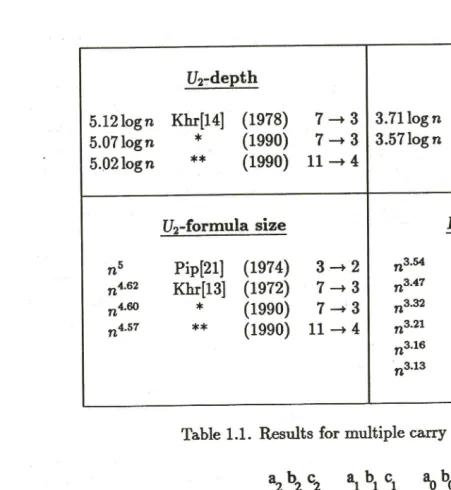
U2-depth B2-depth
5.12 log n Khr[14] (1978) 7 -- 3 3.71 log n * (1990) 3 --► 2 5.07 log n * (1990) 7 • -> 3 3.57 log n ** (1990) 6 -4 3 5.02 log n ** (1990) 11 -4 4
U2-formula size /32-formula size
n' Pip[21] (1974) 3 ---). 2 n3-54 Pip[21] (1974) 3 --,, 2 n4.62 Khr[13] (1972) 7 --, 3 n3A7 Pat[18] (1978) 3 —+ 2
n4-6° * (1990) 7 —+ 3 n3' Pet[20] (1978) 3 —+ 2 n4.57 ** (1990) 11 -+ 4 713'21 * (1990) 3 —+ 2
[image:7.842.71.523.83.574.2]n3.16 ** (1990) 7 -4 3 n3.13 ** (1990) 6 —+ 3
Table 1.1. Results for multiple carry save addition.
a2
b2
c2 al
bl c1
a0b0 c0
Us
Us
• • • FA3 FA3 FA3
0 I
u1 V 1
I V
3 u2 v2 u0 V0
Figure 2.1. Constructing a CSA3.2 using FA3's.
the previously known results even using the same CSA's used by the previous authors. The improvements we get are quite marginal in some of the cases. Our results, however, could only be improved by either designing improved basic carry save adders or by designing circuits which are not constructed from carry save adders.
2. Carry Save Adders
A k-bit full adder (FAk) receives k input bits and outputs flog(k +1)1 bits representing, in binary notation, their sum. Usually k is of the form 2-e — 1.
-o
1
2
3
y1
[image:8.842.71.519.86.252.2](a) (b) (c)
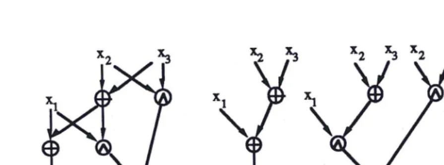
Figure 2.2. An optimal depth implementation of a B2-FA3.
A B2-implementation of an FA3 is given in Fig. 2.2(a). The delay matrix of this FA3 which describes the relative delay of each output with respect to each input is easily seen to be (1 k 2 3 2 32) . The delay characteristics of the CSA 3_,2 obtained are also described by
this delay matrix.
Notice that x1 may be supplied to this FA3 one unit of time after x2 and x3 are supplied, and that yo is obtained one unit of time before yi. Thus, the FA3 can be represented schematically by the 'gadget' appearing in Fig. 2.2(c).
The two formulae obtained by expanding the circuit of Fig 2.2(a) are given in Fig 2.2(b). The formula for yi has size 5. The variable x1 appears only once in it while each of the variables x2, x3 appear twice. We therefore say that the occurrence vector of the formula is (1, 2,2). The occurrence vector of the formula for yo is (1,1,1). Combining these
( 1 2 11 vectors we get that the occurrence matrix of the implementation is
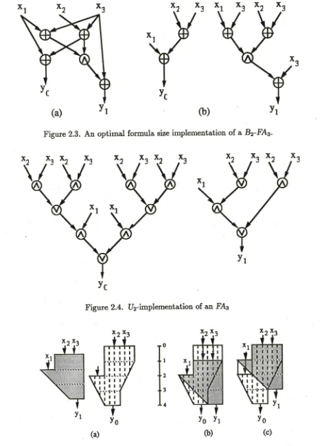
An alternative B2-implementation of an FA3 is given in Fig. 2.3. This implementation
1 2 2 1
has a worse delay matrix (3 3 3) but a better occurrence matrix 3). It can be
checked that no other B2-implementation has a better delay or occurrence matrix than those given.
Both the implementations of Fig. 2.2 and Fig. 2.3 are also minimal with respect to circuit size. This, however, will not happen in general. Since we are not concerned here with the size of the circuits (which will always be 0(n2)) we can think of an implementation of an FA as a set of formulae, one for each output bit. This also stresses the fact that we may try to optimise the structure of each formula separately.
4 3 4)
A U2-implementation of an FA3 is given in Fig. 2.4. It has delay matrix (22 3 and
2 4 4) .
occurrence matrix ( It could be checked that both these are optimal. Note
kl 2 2
x 2 x3 x 2 x3
t
yo
(a)
[image:9.842.79.548.88.737.2](a)
(b)
Figure 2.3. An optimal formula size implementation of a B2-FA3.
Figure 2.4. U2-implementation of an FA3
yo yi yo
(b) (c)
0
i
2
3
4
Using the implementation of Fig. 2.2 we get depth 3.71 log n B2-circuits for carry save addition and using that of Fig. 2.3 we can get 0(70.21) B2-formulae for each output bit of carry save addition. With the implementation of Fig. 2.4 we get depth 5.42 log n U2" circuits and O(n4•70) formulae for carry save addition. These are the best results possible using FA3's. The better results stated in the previous section are obtained using more complicated building blocks.
The construction of the building blocks that are used to get our best results is technically involved. Since we want to concentrate on the general theory we will not describe their construction here. These details will appear in a forthcoming paper. We would just point out here that GSA's could be built using any bit adder, not necessarily using full adders. Our currently best U2 results for example are obtained using a bit adder that
adds 7 bits with weight 1 together with 4 bits of weight 2. It is also not necessary for the result to be supplied in a non-redundant form.
3. GSA-networks
A CSA is regarded henceforth as a black box with k inputs and., outputs (t < k) with the property that the sum of its outputs is always equal to the sum of its inputs. The delay and formula size characteristics of a CSA are described by its x k delay and occurrence matrices.
We assume that all the entries in the delay matrix are positive and that all the entries in the occurrence matrix are at least 1. This corresponds to the assumption that every output depends on every input and that no computation is instantaneous.
A more general setting could allow the outputs to depend on subsets on the inputs. In such cases, —co entries will appear in the delay matrices and 0 entries will appear in the occurrence matrices. Almost all the results of this paper could be extended to cover this more general situation. The complete proofs of these results are much longer however, and although we do need these generalisations in order to get our best results mentioned in Table 1.1 we will not present them here. Some will appear in the planned subsequent paper.
In the sequel, whenever a delay matrix is considered, it is assumed that all its entries are positive and whenever an occurrence matrix is considered it is assumed that all its entries are at least one.
A CSA-network is an acyclic network composed of CSA units of a fixed type. An inductive argument shows that any CSA-network has the property that the sum of its outputs is equal to the sum of its inputs.
Using the delay and occurrence matrices, M and N respectively, of the CSA unit used we can assign a delay and (formula) size to each 'wire' in the network. The inputs to a network are assigned delay 0 and size 1. If the k inputs to a CSA have delays xl, , xk then the i-th output of this CSA will have delay yi = maxi<j<k{nli; si}.
We express this by y = M o x where the o denotes the {max, d-} inner product. If the
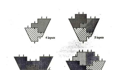
Figure 3.1. Optimal n -k 2 networks for n = 4, 5, 6, 7,8.
delays (respectively, sizes) of its outputs.
Given a fixed CSAk _,1 with delay matrix M and occurrence matrix N, our task is to construct using these units networks with n inputs and £ outputs with minimal delay or formula size. We denote by DM(n) the minimal delay of such an n t network and by
-FN (n) the minimal (formula) size of such a network. Strictly speaking, n t networks exist only if (k — .01 (n — £) (and then use exactly (n —t)1(k — t) GSA's). This is relaxed however by allowing constant zero inputs. Such dummy inputs will also simplify the presentation of the constructions described in Sections 7 and 8.
The optimal networks for some small values of n, constructible using the CSA 3-42 of Fig. 2.2, are shown in Fig. 3.1. For every fixed CSA unit there is a polynomial time
algorithm which constructs for every n the set of n networks with minimal delay. We are interested in the asymptotic behaviour of the functions DM(n) and FN (n). The next theorem states that DM(n) behaves logarithmically and FN (n) polynomially. Theorem 3.1 For every delay matrix M and occurrence matrix N there exist constants 8(M) and e(N) such that
(i) DM (n) = (8(M) o(1)) log n; (ii) FN (n) = nt(N)+°(1).
Proof : By collapsing first the columns then the rows of an n x m array of inputs, we see that
DM(nm) < DM(n) DM (m) DM (i 2).
It follows that the function DM(n) DM(t 2) behaves sub-additively (as its argument
[image:11.842.69.537.69.358.2]argument we get that the limit e(M) = limn„, log FN(n)/ log n exists. These two constants satisfy the required conditions.
Our goal in the next sections will be to determine 8(M) and e(N) as functions of M and N.
4. Lower bounds
Define the following functions :
8'(M) = max{8 > 0 :
e(N) = maxle > 0 :
V x E Rk and y=Afoxi Eil=1 2rils _<EL1 21416
V x E (Rik
IlxIli
i 5_ IINxIlveLemma 4.1 The maxima in the definitions of P(M) and e'(N) exist.
Proof : For every x E Rk and y=Mox let A„ = {6 > 0 : > 2 'i/6 < E 2Yi/s}. It is easy to see that the set A's = Az U {0} is closed. Denote A = nzERk Ax, =
nxERkAiz = A U {0}. The set A', being an intersection of closed sets is also closed. Let m be the maximal entry in M. If we choose x = 0 then yi < m. If 6 E Ao then k = E 2x2 /6 < E n16 < £2m/6 and as a consequence S < m/ log(k/1). Thus A0 and therefore A' are bounded. Thus A' is compact and has a maximum. It is easy to check that max A' > 0 and therefore max A = max A' and their common value is 6'(M). The existence of e'(N) is proved in a similar manner.
More direct proofs for the existence of these maxima could be derived from the arguments used in Sections 5 and 6.
In this section we show that 6'(M), e'(N) are lower bounds for 6(M), e(N). In Sections 5 and 6 we show that they are also upper bounds, thus establishing that 8(M) = 61(M) and e(N) = e'(N).
Theorem 4.2
(i) Dm(n)?_ e(M)log(n/t); (ii) FN(n) > (nlir N).
Proof : Consider an n —+ t network composed of GSA's with delay matrix M. If the inputs to a CSA in the network have delays xl, , sk then the outputs will have delays yi , , yt where y = M o x. The definition of 8 = 61(M) ensures that E",.1 2s;/6 < 2Y.A. Using induction we get a similar relation for the inputs and outputs of the whole network. The n inputs have delay 0. If the outputs all have delay at most d then we get that n < £2`1/6 or equivalently d > S log(n I t).
network. The n inputs have size 1. If the £ outputs all have size at most f then we get
that f > (n/t)`. 0
The argument used in this proof is similar to the one used in a proof that a binary tree of depth t can have at most 21 leaves using Kraft's inequality
(E 2-4 < 1
where the are the depths of the leaves in a binary tree).As an immediate consequence we get
Corollary 4.3
N
61(M) < 5(M); (ii) e(N) 5_ e(N).5. The delay problem
In this section we show that in order to compute SW) we need only consider a finite number of points x E Rk. This provides a practical way of computing 81(M). We will also gain some insight into how a CSA with delay matrix M could be used optimally.
If x E Rk, y E Rt we define
k
Px,y(A) =
E
—E
AYi.J.1 i=1
Lemma 5.1 If max x; < min yi and £ < k then the equation Px,y(A) = 0 has a unique
root A(x, y) in the interval (1, oo).
Proof : If A = 1 then Pz,v(1) = k — t > 0 and if A —* oo then Px,y(A) —oo. Thus the equation has at least one root in the interval (0, oo).
Since a translation of x and y by the same amount leaves the roots invariant, we may assume, without loss of generality that max xi < 0 < min yi. Every positive contribution to Pz,y(A) is now decreasing in A while every negative contribution is increasing. Therefore Pz,y(A) as a whole is decreasing and the uniqueness of the root is
guaranteed. 0
If x E Rk and y E Rt, we denote by y — xT the t x k matrix whose elements are yi — x j. Matrices of this form are called modular. If M', M are two matrices and > mid for every i, j, we say that M' dominates M and we write M' > M.
If we replace S in the definition of 5'(M) by A = 21/6 then since y = M o x implies y — xT > M, we get that e(M) = 1/ log A(M) where
A(m) minf A > 1 xERk ,y Efe,y—xT >M
Ar'< ELi AY'
If M is a delay matrix with positive entries and y—XT > M then clearly maxi xi < mini yi and the uniqueness of A(x, y) follows. We therefore get that E Axi < E A' holds if and only if A > A(x, y). We can thus state the definition of A(M) in the following form
A pair (x, y) of vectors x E Rk and y E Re satisfying y — xT > M will be called a
schedule for M. If we impose the additional requirement that xl = 0 we get a
one-to-one correspondence between schedules and modular matrices dominating M. This set of modular matrices dominating M will be denoted by P(M) and will be called the
modular polyhedron over M.
If M = b — aT is a modular matrix and y — xT > M then y, > maxici<k{bi — a; +xi } =
bi-Fc where c = maxi<;<k{x; —ai}. If we define ei = c-Fa; then we still have y—xiT > M, although x' > x and therefore A(x', y) > A(x, y). Since translating both x and y by the same amount leaves the roots invariant, we may assume that c = 0. So x' = a, y = b, and we have proved the following Theorem.
Theorem 5.2 If M is modular, M = b — aT say, then A(M) = A(a,b).
As an immediate consequence of this theorem we get that
A(M) = max{A(M') : M' E P(M)}.
The set P(M) is defined using a finite set of linear inequalities and it is therefore a polyhedron. As mentioned before, we can identify a point M' E P(M) with the unique
schedule (x, y) which satisfies x1 = 0 and y — xT = M
'
.For every schedule (x, y), define a bipartite graph r(s, y) in which the elements of x and y are the nodes and in which x; and yi are connected by an edge if and only if yi — x; = mii. It is easy to check that (x, y) is a vertex of the polyhedron if and only if the graph P(x, y) is connected. A vertex of a polyhedron is an extremal point of it, that is, a point which is not a convex combination of any other two points in the polyhedron. The polyhedron P(M), has only a finite number of vertices. We denote this finite set of vertices by P*(M). Our aim is to prove that the maximum in the definition of A(M) is attained at some vertex of P*(M).
Suppose that (x, y) E P(M) is not a vertex of P(M), so the graph F(x, y) is disconnected.
We will show that there exists a schedule (x', y') such that r(e, y') is connected and A(x', y') > A(x, y). Suppose that A is the set of variables in the nonempty connected component of P(x, y) containing xl. Let B denote the complementary set of variables. We can break the definition of Px,y(A) in the following way
Px,y(A) =
E
Ax' —E
Ash) +E
Ax' —E
Ain) EA y; EA x1EB yi EBPAN PB(A)
By repeating this procedure we arrive at a schedule for which the graph is connected (so that the schedule corresponds to a vertex of P(M)), without ever decreasing A. We have thus proved
Theorem 5.3 For any delay matrix (with positive entries), A(M) = max{A(M') :
M'
E
P* (M)}In Section 7 we will see that the lower bounds of the previous section are tight. Theorem 5.3 thus says that if M is a non-modular matrix then there exists a modular matrix M' that dominates it (and is a vertex of the modular polyhedron over M) such that asymptotically, we can do as well using M' as we can using M. In Fig. 2.5 we tried to describe the behaviour of a non-modular CSA. The two gadgets in Fig. 2.5(b)(c) turn out to be the vertices of the modular polyhedron. The gadget in (c) turns out to be the optimal. As we noted in Section 2, internal delays are inevitable when using a non-modular gadget. Apriory, it might seem that the ability to delay some of the inputs in some cases and others in other cases is advantageous. This however is not the case. In order to get optimal performance we should always choose the same internal delays. In the example of Fig 2.5, for instance, we should always delay x1 internally and use the gadget shown in (c).
The results of this section could be generalised to cover the case in which a finite set of basic gadgets, each with an associated delay matrix, is given to us. In order to get optimal performance it is always enough to use only one of the available gadgets.
6. The formula size problem
Our aim in this section is to prove that if N is an occurrence matrix and e = e'(N) then there exists a unique direction x
E (Rik
for which 11x111/6 = II II,. Furthermore, allthe components of this direction are strictly positive. The existence of such a positive direction will be needed in Section 8 where constructions achieving the lower bound on formula size from Section 4 are obtained.
We will need the following lemma.
Lemma 6.1 If N is an occurrence matrix then e'(N) > 1.
Proof : It is clear that if N' > N then e'(N') > c'(N). The k x I occurrence matrix 1
all of whose entries are 1 is dominated by every other k x £ occurrence matrix. A direct
computation shows that e (1) = logqi k > 1. 0
We are now ready to prove
Theorem 6.2 If N is an occurrence matrix and e = e'(N) then there exists a unique
direction x E (R>°)k for which
Proof : Consider the function
over the set
B =
E (R+ )k 11x111/e = 1}. The functionf
is continous and theset
B
is compact so the functionf has a
minimal pointx*
inB.
Iff(x*) < 1
we get a contradiction to the requirement that lixliv, < IINxillie for everyx
E (R+)k . Iff(x*) > 1
we get a contradiction to the maximality of 6. Thereforef(x*)
= 1. This establishes the existence of a direction with the required property.In order to prove the uniqueness of
x*,
defineei
= x.1/' and reti = n,1-31t. We now havef(x) = f 1(x1) =
(niiixfi)E)iAand the domain is
B' = {x
E (Rik :Ei xii =
1}. A minimum point off
onB
corresponds to a minimum point of
f'
onB'.
Lemma 6.1 tells us that f > 1. It is well known that for e > 1 theL,
norm, 11xIlt = (Ea isinlic, is strictly convex, that is,!lax + (1 — < allxil, -I- (1 — a)II Yllt for 0 < a < 1, provided that
x
is not a scalar multiple of y. For every i the functionfl(x')
= (reixDt)lif is obtained from 11x11, by scaling and it is therefore also strictly convex. The functionfl(e)
is obtained by summing strictly convex functiOns and it is therefore strictly convex also. The setB'
is convex and thereforef' has
a unique minimum point on it.Finally, we would like to prove that the minimum point
x*
lies in the interior ofB'
so that none of its co-ordinates is 0. LetfAx1)
=[fi(xl)r =
Ei(n'ijej)t. Suppose, on the contrary, that one of the co-ordinates ofx* is
0. We know of course that at least one of the co-ordinates ofx*
is non-zero. Without loss of generality assume that xi = 0,x; > 0.
It is easy to check that the function (niiA)e (ni2(x2 — Ant has a negative derivative at A = 0. For small values of A we would therefore get that
ff(4)
<ff(x*),
or equivalentlyMel)
<fl(x*),
where4 = (A, x2 —
A, ,x,„).
Since this holds for every i we get that for sufficiently small A,f'(4)
<f(x*)
which contradicts the minimalityof
x*.
0The strict convexity of the functions involved makes the numerical task of finding = e' (N) and the direction
x = x(N)
satisfying 11x111/, = iiNx hie a very easy one. As we shall see in Section 8, the components of the directionx(N)
give the ratios between the sizes of the inputs that should be fed into this gadget if it is to be used optimally.7. Depth constructions
As we saw in Section 5, for every delay matrix
M
there exists a modular delay matrixM'
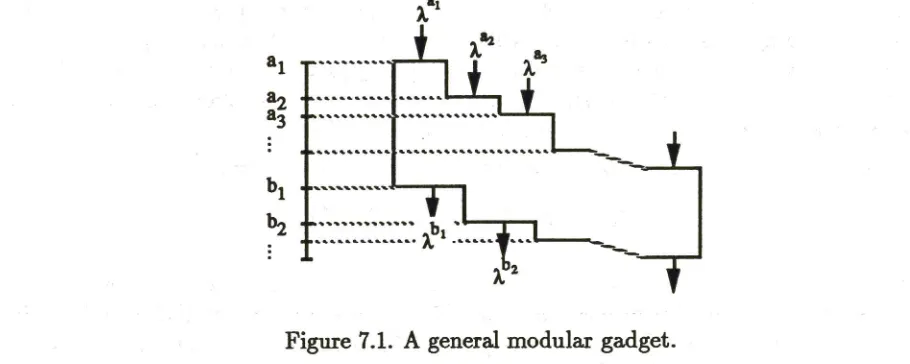
which dominates it and for which A(M) = A(M'). It is therefore enough to consider in this section only modular gadgets. A general modular gadget is shown in Figure 7.1. It has the modular delay matrixM = b — aT
where we assume that 0 = al < a2 < ak < bi < b2 < <bt
and <k.
We assume here that all the outputs are produced after all the inputs were supplied which is always the case if all the entries in the delay matrix are positive. As mentioned in Section 3, the results of this section could be extended to cover more general cases but we shall not do so here. The characteristic equation of this gadget isa2
al
a2 a3
bi
b2 bbl '
[image:17.842.66.521.84.266.2]2
Figure 7.1. A general modular gadget.
We know that this equation has a unique root in the interval (1, oo) which we denote by A = A(a,b).
Our goal in this section is to prove the following theorem
Theorem 7.1 If M = b— aT is a modular delay matrix then DM (n) < (1 + o(1)) logy n
where A = A(a, b).
This immediately gives us
Corollary 7.2 For every delay matrix M
V x E Rk and y=Mox
S(M) = (M) = max{S > 0 :
E2zi 15
.i
< a
i
2V`16}.
Proof (of Theorem 7.1) :
We first consider an important special case. Case 1. The elements of a, b are integral.
A CSA is said to lie at level d in a network iff its inputs are supplied at times
d al, , d + a k. Its outputs are then available at times d b , d bt. Since
we assume here that all the delays are integral we only have to consider integral levels. We can describe the essentials of a network by specifying the number Cd of level-d GSA's used in it. The balance of the number of signals generated and consumed at time d is given by
Bald =
E
Cd-a,E
Cd-b, •j=1 i=1
consumed generated
If Bald > 0 then the network accepts Bald new inputs at time d. If Bald < 0 then the network yields IBaldI outputs at time d. Note that any network specified in such a way uses every signal immediately after it is generated.
The number of signals processed at time d is anA-d where a =
E
Aai =E
Abi. The number of signals processed at time 0 is therefore 0(n) and the number of signals processed at time log), n is 0(1). This however does not correspond to a concrete construction for two reasons. First, the above process is infinite, it begins at time -oo and never ends. Secondly, the number of gadgets that should be used at each time unit is generally not integral. These problems are however easily overcomed.We choose
C - rnA-d cl
d 0
if 1 < nA-d < n, otherwise,
where c = (1-1)/(k-,).
We now verify the following facts.
(i) If 0 < d < th then
Bald = E irotai-d + cl > n.1-d,
aj <d
so we may input at least n inputs at time 0, and even some more at times 1,...,ak.
(ii) If lh < d < Llog A n] then
Bald .2. EinAaj-d
+ —
ELnabi-d+Clj=1 i=1
> (71A-d Aci.0 kc - (n.\ -d EAbo — t(c + 1)
j=1 i=1
= kc - t(c +1) = -1.
Since Bald is integral we get that Bald > 0. In other words no outputs are produced at times less than or equal to [logy nj
(iii) If I Jog), n j < d < [log), nj bt then
Bald > - E C d—bi i=1
> EinAbi _d
i=1
> —A-di > Ab. — f(c + 1) where di = d - ilogi n-1 .
i=1
We therefore get a total of at most L = Al El=i A 1'1 ibt (c + 1) outputs at
times less than or equal to LlogA nj N. Note that L is fixed, independent of n.
A final stage could now be used to reduce the L outputs obtained to only 1. Thus, if a, b are integral then we even have DM(n) < log), n + 0(1).
Note that without the assumption that al < a2 < < ak < bl < < b1 this construction may fail. It will not always be guaranteed that Bald > 0 for 1 < d < b1.
Case 2. The elements of a, b are arbitrary positive real numbers.
Consider the integer schedule
= (Lqad , Lqad , ,
b = (1011 , 1021, - • ,
where q = q(n) oo as n oo. Note that X = A(Ti,b) Alh as q —+ co. The
construction given in Case 1 produces L = 0(q) outputs, all within time [logs +It = q(logA n +0(1)). Reducing the timescale in this construction by a factor of q throughout, produces a network of delay log), n + 0(1) with O(q) outputs. The final stage to reduce these outputs to t requires a delay of 0(log q). This construction satisfies the Theorem provided that q is chosen so that log q = o(log n).
8. Formula size constructions
Let N be an occurrence matrix with entries greater than or equal to one. Choose a vector x E (0, oo)k and define the following two vectors
ai = log xi 1 < j < k, bi = log Mi niix; 1 < i < t.
Associate with every CSA with occurrence matrix N a delay matrix M(x) = b — aT
.
Note that all the entries of M(x) are positive.Suppose that is a network composed of GSA's with occurrence matrix N, and therefore with delay matrix M(x). To every wire w in
r
we can now assign both a size f(w) and a delay d(w). We can generalise the observation that the size of a formula is at most 2 to the power of its depth.Lemma 8.1 For any wire w in r we have f(w) < 2d(w).
Proof : If w is an input wire then f(w) = 1 and d(w) = 0 so the relation holds
with equality. Suppose now that u1,... , uk are the inputs of some CSA in the network, that f(u;) < 2d(u3) for every j, and that , are the outputs of this CSA. Let t = maxi{d(u;) — ai }. Then t may be regarded as the time at which this CSA is activated. The delays of the inputs satisfy d(u;) < t a; while the delays of the outputs satisfy d(vi) = t bi. The size of vi will now be
Atli) < E ni j2t+aj = 2t \---, = 2t+bi = 2d(vi).
f(vi) =
E
ni; f (u;) <Enii2
La
niix;i i .i
Thus the claim of the lemma follows by induction. o
section give (n 1)-networks composed of GSA's with delay matrix M = M(x) (and occurrence matrix N) with depth (8(M) + o(1)) log n. Using the previous Lemma we get that these networks have formula size n6(M)+o(1)
Finally, noticing that if = then M = M(x) satisfies 5(M) = 8'(M) =
e(N) we get
Theorem 8.2 For every occurrence matrix N we have FN(n) < ne(N)+0(1).
An immediate consequence is the following result.
Corollary 8.3 For every delay matrix N
e(N) = e(N) = max{e > 0 : V x E (R+)k, 11x111/,
9. Numerical examples
The delay matrix of the FA3 described in Fig. 2.1 is the modular matrix M = (2 3)T — (1 0 0). Therefore A(FA3) is the unique positive root of the cubic equation A3 -I- A2 — A — 2 = 0. We can verify that A 1.2056 and that logy nL•,_ 3.71 log n.
The delay matrix of the FA3 described in Fig. 2.4 is the non-modular matrix (22 43 43 ).
The two vertices of the modular polyhedron are (22 44 44) = (4 4)T — (2 0 0) and
4
3 `) = (4 3)T — (1 0 0) (compare with Fig. 2.5). The characteristic equation of
the first vertex is 2A4 — A2 — 2 = 0 and its solution is Al = 1.1317. The characteristic equation of the second vertex is A4 + A3 — A — 2 = 0 and its solution is
A2 1.1365. The second posibility is clearly better and the circuits that we would build would have depth log),, n 5.42 log n.
4 6 6 6
Khrapchenko [14] designed a U2-FA7 with delay matrix ( 6 5 6 6 7 7 7 7) . 6 6 Using
5 6 6 6 6 6 6
ad hoc methods he was able to construct with it networks of depth 5.12 log n. The delay matrix of Khrapchenko's FA7 is non-modular. The optimal vertex in the modular
(5 6 6 6 6 6 6
polyhedron of this matrix is 6 7 7 7 7 7 7) and therefore a(FA7 ) is the unique 5 6 6 6 6 6 6J
positive root of the equation A7 + 2A6 — A — 6 = 0. We find that A 1.1465 and that log), n 5.07 log n. We can thus improve Khrapchenko's construction even using his own gadget. We can reduce the depth of the U2-circuits to 5.02 log n using a novel design of a CSA 11-44.
The size of the optimal formulae for multiple carry save addition that can be obtained using GSA's based on the FA3 described in Fig. 2.2 is n'+'(1) where
1 Vxi, X2, X3 > 0
e = max S :
p xip + 4 + 4 < (x, + x2 + x3)P + (x1 + x2 + 3x3)P
10. Concluding remarks
Many related open problems still remain. The hardest of them all is probably to determine the exact depth and formula size of multiplication, multiple addition and multiple carry save addition. In this paper upper bounds on these complexities were obtained. Although these bounds may be close to the real values, we believe that they may be further improved by devising better basic building blocks.
A more tractable problem, perhaps, is the question of whether or not the optimal depth and formula complexities of the above mentioned problems can be obtained, or at least approached, using carry save networks.
References
[1] Aho A.V., Hoperoft J.E., Ullman J.D., The design and analysis of computer algorithms. Addison-Wesley, 1974.
[2] Avizienis A., Signed-digit number representation for fast parallel arithmetic. IEEE Trans. Elec. Comp. Vol. EC10 (1961), pp. 389-400.
[3] Brent R., On the addition of binary numbers. IEEE Trans. on Comp., Vol. C-19
(1970), pp. 758-759.
[4] Brent R., Kuck D.J., Maruyama K., The parallel evaluation of arithmetic expressions without division. IEEE Trans. on Comp., Vol. C-22 (1973), pp. 532-534.
[5] Chin A., Shallow circuits for the counting functions. To appear in Information
Processing Letters.
[6] Dadda L., Some schemes for parallel multipliers. Alta Frequenza, Vol. 34 (1965),
pp. 343-356.
[7] Dadda L., On parallel digital multipliers. Alta Frequenza, Vol. 45 (1976), pp.
574-580.
[8] Dunne P.E., The complexity of Boolean networks. Academic Press, 1988.
[9] Karatsuba A., Ofman Y., Multiplication of multidigit numbers on automata. Soviet Physics Dokl., Vol. 7 (1963), pp. 595-596.
[10] Khrapchenko V.M., Asymptotic estimation of addition time of a parallel adder.
Problemy Kibernet., Vol. 19 (1967), pp. 107-122 (in Russian). English translation
in Syst. Theory Res., Vol. 19 (1970), pp. 105-122.
[11] Khrapchenko V.M., Complexity of the realization of a linear function in the class of
7r-circuits. Mat. Zametki, Vol. 9 (1971), pp. 35-40 (in Russian). English translation
in Math. Notes Acad. Sciences USSR, Vol. 9 (1971), pp. 21-23.
[12] Khrapchenko V.M., Methods of determining lower bounds for the complexity of
r-schemes. Mat. Zametki, Vol. 10 (1972), pp. 83-92 (in Russian). Math. Notes Acad. Sciences USSR, Vol. 10 (1972), pp. 474-479 (English translation).
[13] Khrapchenko V.M., The complexity of the realization of symmetrical functions by
in Mathematical Notes of the Academy of Sciences of the USSR Vol. 11 (1972) pp.
70-76.
[14] Khrapchenko V.M., Some Bounds for the Time of Multiplication. Problemy
Kibernet., Vol. 33 (1978), pp. 221-227 (in Russian).
[15] Knuth D.E., The art of computer programming, Vol. 2, Seminumerical algorithms
(second edition). Addison-Wesley.
[16] Mehlhorn K., Preparata F.P., Area-Time Optimal VLSI Integer Multiplier with
minimum computation time. Information and Control, Vol. 58 (1983), pp. 137-156.
[17] Ofman Y., On the algorithmic complexity of discrete functions. Doklady Akadernii
Nauk SSSR, 145 pp. 48-51 (in Russian). English translation in Soy. Phys. Doklady, Vol. 7 (1963) pp. 589-591.
[18] Paterson M.S., New bounds on formula size. Proc. of 3rd GI conference on
Theoretical Computer Science 1977, Lecture Notes in Computer Science 48, Springer-Verlag 1977, pp. 17-26.
[19] Paterson M.S., Pippenger N., Zwick U., Faster circuits and shorter formulae for
multiple addition, multiplication and symmetric Boolean functions. Proceedings of the 31st FOCS, St. Louis 1990.
[20] Peterson G.L., An Upper Bound on the size of formulae for symmetric Boolean
functions. Technical Report No. 78-03-01, University of Washington.
[21] Pippenger N., Short formulae for symmetric functions. IBM report RC-5143,
Yorktown Heights, NY (November 20, 1974).
[22] Pratt V.R., The effect of basis on size of Boolean expressions. Proc. 16th IEEE
Symposium on FOGS (1975), pp. 119-121.
[23] Preparata F.P., Muller D.E., Efficient parallel evaluation of Boolean expressions.
IEEE Trans. Comp., Vol. C-25 (1976), pp. 548-549.
[24] Schonhage A., Strassen V., Schnelle Multiplikation grosser Zahlen. Computing,
Vol. 7 (1971), pp. 281-292.
[25] Spira P.M., On time-hardware complexity tradeoffs for Boolean functions. Proc. 4th
Hawaii Int. Symp. on System Sciences (1971), pp. 525-527.
[26] Valiant L.G., Short monotone formulae for the majority function. Journal of
Algorithms, Vol. 5 (1984), pp. 363-366.
[27] Van Leijenhorst D.C., A. note on the formula size of the "mod k" functions. Info.
Proc. Letters, Vol. 24 (1987) pp. 223-224.
[28] Wallace C.S., A suggestion for a fast multiplier. IEEE Trans. Electronic Comp.
EC-13 (1964) pp. 14-17.
[29] Wegener I., The complexity of Boolean functions. Wiley-Teubner Series in Computer