A Knowledge-Light Approach to Regression
using Case-Based Reasoning
Neil McDonnell
A thesis submitted to the University of Dublin, Trinity College in fulfilment of the requirements for the degree of
Doctor of Philosophy
Declaration
I, the undersigned, declare that this work has not previously been submitted to this or any other University, and that unless otherwise stated, it is entirely my own work. This thesis may be borrowed or copied upon request with the permission of the Librarian, University of Dublin, Trinity College. The copyright belongs jointly to the University of Dublin, Trinity College and Neil McDonnell.
Neil McDonnell
Acknowledgements
I would like to thank a number of people who have helped me in various ways over the past three years. Without their assistance, this thesis would certainly not have seen the light of day.
First, let me express my gratitude to my supervisor, Professor Pádraig Cunningham. His clear technical direction was invaluable in guiding me to a productive research path when I was struggling to find my bearings. He was unfailingly generous in his encouragement and support, and kind enough to administer a gentle push when it was most needed.
Second, I would like to thank my colleagues in the Machine Learning Group in Trinity College Dublin, both past and present. These include Lorcan Coyle, Marco Grimaldi, Sarah Jane Delany, John Loughrey, Conor Nugent, Dónal Doyle, Mike Carney, Ken Bryan, Derek Greene, Deirdre Hogan, Michael Davy and Alexey Tsymbal. It has been a pleasure to work with them, and I am constantly impressed by the dedication and expertise they bring to their research.
Third, thanks to my colleagues in the University of Ulster who have worked with me under the North-South Cooperation Programme. Our frequent meetings helped me crystallise many of the ideas that are presented in this thesis.
Finally, I owe a special thanks to my wife, Edel, for everything she has done for me over the years. This thesis is dedicated to her.
Neil McDonnell
Abstract
Case-based reasoning (CBR) is among the most influential paradigms in modern machine learning. It advocates a strategy of storing specific experiences in the form of cases, and solving new problems by re-using solutions from similar past cases. The most difficult aspect of CBR is deciding how to adapt past solutions to precisely match the circumstances of new problems. No generally applicable method of doing this has been found; different domains and tasks have their own individual characteristics, and successful adaptation has usually relied on the presence of explicit, hand-coded domain knowledge. Such knowledge is usually difficult both to acquire and maintain. For this reason, most CBR systems in operation today are ‘retrieval only’ in that they do not attempt to adapt the solutions of past cases to solve new problems.
For certain machine learning tasks, however, customisation of old solutions can be performed using only knowledge contained within the set of stored cases. One such task is regression (i.e. predicting the value of a numeric variable). Regression is among the oldest machine learning tasks, dating back to Francis Galton’s work on predicting the heights of parents and their children in nineteenth century England. A modern example would be to predict tomorrow’s stock market prices based on today’s financial data. Many different approaches to solving regression problems have been developed over the years, for example,
k-NN, locally weighted linear regression and artificial neural networks.
The aim of this thesis is to apply CBR to the problem of regression. It begins by analysing previous attempts to do this, paying particular attention to those aspects that might be improved. One CBR-based approach from the mid-1990’s is examined in considerable detail. It works by finding the differences between a new problem and a similar past problem, then searching for a pair of stored cases with the same differences between them. These stored cases indicate the effect of the differences on the solution. This ‘case differences’ approach has much to recommend it. In particular, the knowledge needed to solve new problems is automatically generated from stored cases—no additional external knowledge must be added. Unfortunately, it also suffers from some theoretical limitations that greatly restrict its use.
Contents
Acknowledgements ...iii
Abstract... iv
Contents... vi
List of Figures... ix
List of Tables... xi
Chapter 1 Introduction... 1
1.1 Case-Based Reasoning... 2
1.2 Locally Weighted Linear Regression... 3
1.3 Problem Statement... 3
1.4 Contributions of this Thesis... 4
1.4.1 Analysis of previous research... 4
1.4.2 Presentation of new CBR-based regression algorithms... 4
1.4.3 Implementation and evaluation of a prototype system ... 5
1.5 Publications Related to this Thesis ... 5
1.6 Summary and Structure of this Thesis... 5
Chapter 2 Regression... 7
2.1 Linear Regression ... 8
2.2 k-Nearest-Neighbour (k-NN) ... 10
2.3 Locally Weighted Linear Regression (LWLR)... 13
2.4 Which Regression Algorithm to Use? ... 16
2.5 Use of Regression Algorithms in this Thesis... 16
2.5.1 Model trees ... 17
Chapter 3 Case-Based Reasoning... 20
3.1 Advantages of CBR ... 21
3.1.1 Simpler system construction and maintenance... 21
3.1.2 Improved performance during operation... 23
3.1.3 When to use CBR ... 25
3.2 CBR Problem Solving Methodology... 26
3.2.1 Construction phase... 28
3.2.2 Operation phase ... 36
3.3 Knowledge Contained Within a CBR System... 37
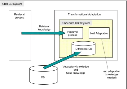
3.4 Case Study: CBR-CD ... 39
3.5 Summary... 41
Chapter 4 Using CBR for Regression ... 42
4.1 CBR-B Algorithm... 43
4.1.1 Problem solving methodology... 43
4.1.2 Advantages and limitations... 44
4.2 CBR-D Algorithm... 46
4.2.1 Problem solving methodology... 47
4.2.2 Advantages and limitations... 50
4.3 CBR-AR Algorithm... 51
4.3.1 Problem solving methodology... 52
4.3.2 Advantages and limitations... 55
4.3.3 Prior research on using case differences for adaptation... 59
4.4 Discussion... 60
4.5 Summary... 62
Chapter 5 Case-Differences Regression Algorithm (CBR-CD)... 63
5.1 Introduction to Case Differences ... 63
5.1.1 Constructing an embedded CBR system to use for adaptation... 64
5.1.2 First attempt at using case differences to make a prediction ... 65
5.1.3 Problems associated with naïve application of case differences... 67
5.2 Problem Solving Methodology of CBR-CD... 68
5.2.1 Using LWLR to help choose difference-cases ... 68
5.2.2 Using LWLR to reduce prediction error... 83
5.2.3 Combining multiple predictions to reduce prediction error... 85
5.2.4 Adding support for non-numeric attributes ... 86
5.3 Advantages and Limitations of CBR-CD ... 90
5.4 Possible Extensions to CBR-CD... 91
5.4.1 Constructing adaptation paths from several difference-cases... 91
5.4.2 Normalizing numeric difference vectors ... 93
5.5 Summary... 95
Chapter 6 Implementation of CBR-CD ... 97
6.1 Architecture of CBR System ... 97
6.2 CBR-CD Implementation Notes... 100
6.2.1 Parameters for the construction phase ... 100
6.2.2 Parameters for the operation phase... 101
6.3 Summary... 103
Chapter 7 Experimental Evaluation ... 104
7.1 Datasets Used for Experimental Evaluation ... 104
7.2 Overview of Experiments ... 107
7.3 Experiment 1—Comparing Different Variants of CBR-CD... 108
7.3.1 Experiment 1: Experimental setup... 108
7.3.2 Experiment 1: Results... 109
7.3.3 Experiment 1: Conclusions... 112
7.4 Experiment 2—Comparing Different Regression Algorithms ... 113
7.4.1 Experiment 2: Experimental setup... 113
7.4.2 Experiment 2: Results... 115
7.4.3 Experiment 2: Conclusions... 118
7.4 Discussion... 120
7.5 Summary... 121
Chapter 8 Conclusions and Future Work... 123
8.1 Thesis Summary... 123
8.1.1 Introduction to regression and CBR (Chapters 2 & 3) ... 123
8.1.2 Previous approaches to using CBR for regression (Chapter 4) ... 124
8.1.3 New CBR-based regression algorithms (Chapters 4 & 5)... 125
8.1.4 Implementation and evaluation of new algorithms (Chapters 6 & 7)... 125
8.2 Conclusions... 126
8.4 Future Work... 127
List of Figures
Figure 2.1: Examples of linear and non-linear regression models... 8
Figure 2.2: Predicting a numeric value using k-NN... 13
Figure 2.3: Predicting a numeric value using LWLR... 15
Figure 2.4: Regression algorithms used in this thesis... 17
Figure 2.5: Model tree and linear models for the Servo dataset ... 18
Figure 3.1: Construction and operation of a CBR system ... 28
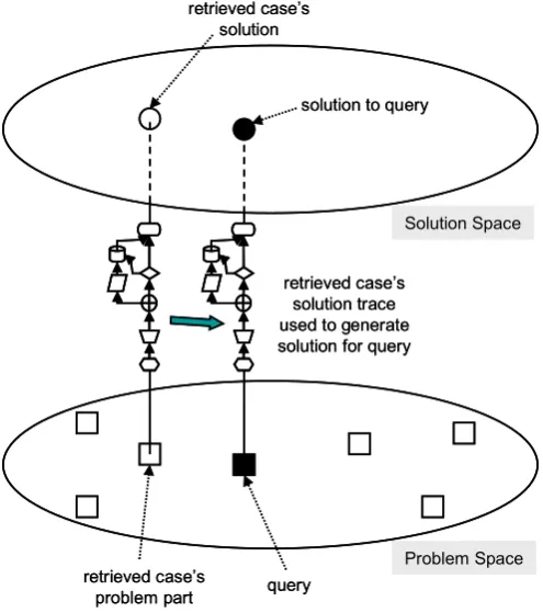
Figure 3.2: The CBR adaptation process ... 32
Figure 3.3: Null adaptation ... 33
Figure 3.4: Transformational adaptation... 34
Figure 3.5: Generative adaptation... 35
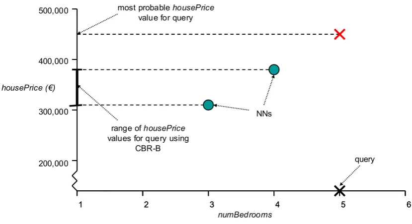
Figure 4.1: Adaptation process for CBR-B... 44
Figure 4.2: Inability of CBR-B to take case positions into account... 46
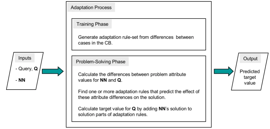
Figure 4.3: Adaptation process for CBR-D ... 48
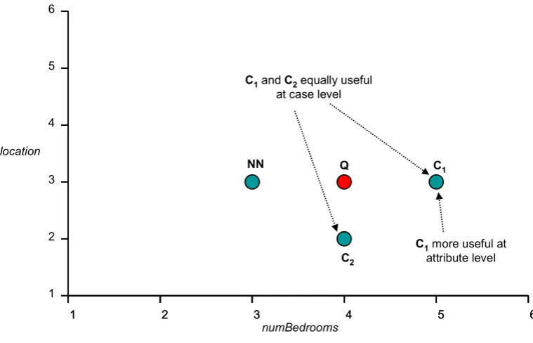
Figure 4.4: Advantage of considering diversity at attribute level... 50
Figure 4.5: Adaptation process for CBR-AR... 54
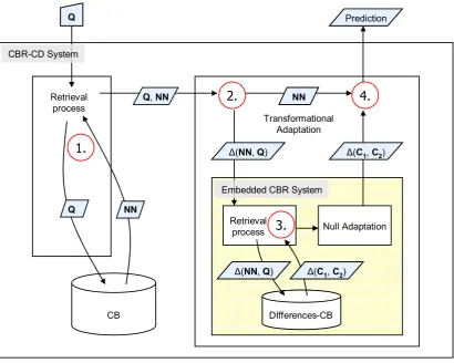
Figure 5.1: Structure of a CBR-CD system ... 65
Figure 5.2: Solving a query using case differences ... 66
Figure 5.3: Flow of data through a simplified CBR-CD system during problem solving... 67
Figure 5.4: Using gradients to help find a useful difference-case (Approach 2) ... 70
Figure 5.5: Relationship between difference-cases and gradients ... 74
Figure 5.6: Approach 3: combining difference-cases and gradients in a vector... 76
Figure 5.7: Validity of Approach 3 for arbitrary target functions... 77
Figure 5.8: Approach 4: combining difference-cases and gradients in a scalar... 78
Figure 5.9: Assessing difference-cases using Approach 4... 79
Figure 5.10: Assessing difference-cases using Approach 3... 80
Figure 5.12: Using LWLR to avoid noisy cases... 84
Figure 5.13: Making a prediction using CBR-CD ... 89
Figure 5.14: Using adaptation paths to bridge the gap between the query and an NN... 92
Figure 5.15: Equivalent difference-cases of different length... 94
Figure 6.1: Class diagram for CBR system... 99
Figure 7.1: Experiment 1—Results for Boston Housing dataset... 110
Figure 7.2: Experiment 1—Results for Tecator dataset... 110
Figure 7.3: Experiment 1—Results for Abalone dataset ... 111
Figure 7.4: Experiment 1—Results for CPU dataset ... 111
Figure 7.5: Experiment 1—Results for Servo dataset... 112
Figure 7.6: Experiment 1—Aggregated Results... 112
Figure 7.7: Experiment 2—Results for Boston Housing dataset... 115
Figure 7.8: Experiment 2—Results for Tecator dataset... 116
Figure 7.9: Experiment 2—Results for Abalone dataset ... 116
Figure 7.10: Experiment 2—Results for CPU dataset ... 117
Figure 7.11: Experiment 2—Results for Servo dataset... 117
List of Tables
Table 4.1: CBR-based regression algorithms ... 42
Table 4.2: Problem solving capabilities of CBR-based regression algorithms... 60
Table 4.3: Requirements for a new CBR-based regression system ... 61
Table 7.1: Datasets used for experimental evaluation ... 105
Table 7.2: Values of parameters set automatically in CBR-CD ... 108
Table 7.3: Values of k used by CBR-B and CBR-D... 115
Table 7.4: CBR-D vs. CBR-B... 118
Chapter 1
Introduction
The field of Machine Learning looks at ways in which computer systems can learn from past experiences [Mitchell 1997, p. xv]. Most computer systems do not display this ability, but instead have their behaviour fully defined before they enter operation. All knowledge necessary for carrying out their tasks is pre-programmed; situations not catered for are viewed as specification and/or design failures, to be remedied by corrections in which the missing functionality is added. This approach is appropriate in circumstances where a system’s inputs, outputs, and operating environment can be fully specified in advance. Imagine, for example, a system that accepts the votes from an election in a particular format, counts them according to a defined set of rules, and outputs a set of results. Assuming that everything is designed correctly, the system will display 100% competence in its task from the moment of deployment.
Unfortunately, a complete specification of this kind is not always available (or possible). Suppose, for example, that we are asked to construct an online customer support system that helps customers find solutions to problems they encounter while attempting to assemble an item of furniture. The range of problems that may arise cannot be fully specified in advance. What is needed is a system that initially offers assistance for what are anticipated to be the most common problems, and that expands its expertise based on the range of problems presented by users over time. This can be achieved by regular updates to the system by its human designers. Alternatively, the system can update itself by incorporating a machine learning element that learns from its experiences in some way. This element might accept discrete user sessions in a pre-defined format and use them to improve the system’s response when faced with similar situations in the future.
assumed to be one of a number of standard Artificial Intelligence tasks. Regression (i.e., predicting the value of a numeric variable) is among the most fundamental of these, both in its own right and as a sub-component of more complex tasks [Campbell at al. 2000]. Sample regression applications include predicting tomorrow’s temperature based on today’s meteorological data, or predicting a person’s blood pressure based on lifestyle details.
This thesis focuses on the problem of regression in machine learning. It describes a generic framework for accepting prior experiences and using them to predict the value of some numeric variable. In principle, these prior experiences can take any form. In practice, however, they can usually be represented as a set of records in a database, each containing a number of well-defined fields. We will assume that prior experiences are available in this form, and that at least one data field has a numeric type. The two primary technologies used to construct this framework are case-based reasoning [Aamodt and Plaza 1994; Kolodner 1992] and locally weighted linear regression [Atkeson at al. 1996].
1.1 Case-Based Reasoning
In case-based reasoning (CBR) systems, prior experiences are stored as a set of cases in a case base (CB). New problems are solved by re-using solutions from similar, previously solved cases. Each case generally has a problem part that describes the problem to be solved, and a solution part that details the solution eventually applied. In this thesis, the problem part is assumed to consist of a set of problem attributes (at least one of which is numeric), with the solution part comprising a single numeric solution attribute.
A new case to be solved is often called a query case. Given values for its problem attributes, the system’s task is to predict the value for its solution attribute (also referred to as the target value). The problem solving process involves retrieving prior cases that are similar to the query, and re-using their solutions in some way.
CBR systems have been described as lazy and local—lazy in that the process of generalizing from past experiences is deferred until a query is received, and local in that only those cases most similar to the query are used to provide a solution. This approach contrasts with that of
eager, global learners such as neural networks, where all prior experiences are compiled into a global model during an initial training phase and this model is then used to predict solutions for new problems.
1.2 Locally Weighted Linear Regression
Locally weighted linear regression (LWLR) is another lazy, local approach to regression. Each problem is represented as a set of numeric attributes. When a new problem is received, similar past problems are retrieved and used to construct a linear model in multi-dimensional domain space. This model is than used to predict a solution.
LWLR is one of a number of standard algorithms that are commonly used to tackle regression problems. Although computationally expensive, it tends to perform well in domains where all relevant aspects of a problem can be represented by numeric attributes. Chapter 2 describes LWLR in greater detail.
1.3 Problem Statement
Regression is among the most important problems in machine learning. CBR is among the most important techniques in modern Artificial Intelligence [Aha 1998]. The goal of this research is to combine the two by using CBR to solve regression problems. In particular, it aims to develop a regression system that demonstrates the following capabilities:
Prior experiences are stored as a set of cases, where each case is represented by a set of problem attributes—at least one of which is numeric—and a numeric solution attribute. New query cases are solved by retrieving similar past cases and re-using their
solutions.
Prediction accuracy matches or exceeds that of alternative regression techniques on a range of standard real-world datasets.
The aim of this research can be summed up as follows:
1.4 Contributions of this Thesis
The principal contributions of this thesis are as follows:
1. Previous research into the use of CBR for regression is critically analysed. Shortcomings in previous approaches are identified and discussed, and inform the requirements for an improved approach.
2. Two new CBR-based regression algorithms are presented. The first is a minor variant of k-NN in which diversity among nearest neighbours is preferred. The second aims to address the limitations of previous approaches and is more complex and robust.
3. A working CBR-based prototype is implemented that provides accurate, robust performance.
1.4.1 Analysis of previous research
The traditional approach to solving regression problems using CBR has been to apply a modified k-NN algorithm (for an introduction to k-NN, see [Mitchell 1997, Chapter 8]); predictions are made by taking the weighted average of solutions from past cases similar to the query. An alternative approach that uses the differences between stored cases to generate a set of adaptation rules was proposed in the late 1990’s [Hanney and Keane 1996, 1997; McSherry 1998]. This approach contained much that was promising, but was hampered by theoretical limitations that made it unsuitable for use in real-world domains. Evaluations of the technique were therefore restricted to artificial datasets.
This thesis examines these previous approaches to performing regression using CBR. It looks in detail at the algorithm proposed by Hanney and Keane, at its limitations and the attempts made to solve them. These limitations lead directly to a set of requirements for an improved approach.
1.4.2 Presentation of new CBR-based regression algorithms
used as a heuristic to determine which stored cases are most likely to be useful for solving each individual query.
1.4.3 Implementation and evaluation of a prototype system
The two new regression algorithms were fully implemented and evaluated on a number of standard datasets. Results show that they perform well relative to alternative regression techniques.
1.5 Publications Related to this Thesis
McDonnell, N. and Cunningham, P.: 2006, A Knowledge-Light Approach to Regression using Case-Based Reasoning, Proceedings of the 8th European Conference on Case-Based Reasoning (ECCBR 2006), pp. 91–105, Springer.
McDonnell, N. and Cunningham, P.: 2005, Using Case Differences for Regression in CBR Systems, Proceedings of the 25th Annual International Conference of the BCS SGAI (AI-2005), pp. 219–232, Springer.
1.6 Summary and Structure of this Thesis
In brief:
Chapter 2 examines the problem of regression and some traditional approaches to solving it. Chapter 3 introduces CBR and describes its characteristics and problem solving methodology. Chapter 4 shows how CBR can be applied to regression, and introduces a new algorithm that is a variant of k-NN. Chapter 5 introduces a second new algorithm for performing regression using CBR. Chapter 6 describes the implementation of the two new algorithms, and Chapter 7 evaluates their performance relative to alternative approaches. Chapter 8 finishes by presenting some conclusions and possibilities for future work.
In more detail:
Chapter 3 begins with a presentation of the principles of CBR, the primary technology underlying this research. The process of constructing and operating a CBR system is examined in detail, and the different types of knowledge contained within a CBR system are identified.
Chapter 4 looks at three different ways in which CBR can be used to solve regression problems. The first makes predictions by taking the weighted average of solutions to past cases similar to the query. The second is a new variant that aims for diversity among the cases used for each prediction. The third is that taken in [Hanney and Keane 1996, 1997], and involves generating adaptation rules from the differences between past cases. The limitations of this approach motivate the new algorithm described in Chapter 5.
Chapter 5 constitutes the central part of this thesis. It takes a bottom-up approach to describing a new algorithm for performing regression using CBR. The basic ideas are presented first, then enhancements and modifications are made until the final algorithm is complete. The chapter concludes by examining some potential enhancements to the algorithm that failed to provide improved performance in practice.
Chapter 6 looks at the implementation of a prototype CBR system that includes the regression algorithms described in Chapters 4 and 5.
Chapter 7 evaluates the performance of the two new regression algorithms relative to alternative techniques.
Chapter 2
Regression
All computer systems have a particular task and a set of technologies for achieving it. This research involves constructing a system whose task is regression (i.e., predicting the value of a real-valued numeric variable). The term ‘regression’ was first used by Francis Galton in the nineteenth century [Galton 1886]. He found that the heights of children with exceptionally tall or short parents tended towards the societal mean, and referred to this phenomenon as ‘regression towards mediocrity’. Graphing the mean heights of parents and children produced a straight line. This became known as a regression line, and the process of fitting data to such lines as regression [Bland and Altman 1994].
Figure 2.1: Examples of linear and non-linear regression models (linear model from [Bland and Altman 1994]; non-linear model from [Motulsky1999])
Many different approaches to the regression task have been used over the years (see [Uysal and Güvenir 1999] for an overview). The earliest (beginning with Galton) involved fitting data to a simple linear model; this will henceforth be referred to as linear regression. Other approaches include the possibility of modelling non-linear as well as linear relationships. These include non-linear regression [Seber and Wild 1989], locally weighted linear regression,
k-NN, neural networks [Lippmann 1987], radial basis function networks [Orr 1996], regression trees [Breiman et al. 1984], and model trees. Those that have direct relevance for this research are linear regression, k-NN, and locally weighted linear regression.
2.1 Linear Regression
Linear regression estimates the expected value of one numeric variable given the values of one or more others [Draper and Smith 1998]. Many different terms are used for these variables; we will refer to them as the solution and problem attributes respectively. Linear regression is ‘linear’ in that solution y is assumed to be a linear combination of problem attributes
a1, a2, …, an:
a a an
where is the intercept and is a random error*. Given problem attribute values
(v1, v2, …, vn) for a new problem, a linear model can be used to predict its target value yˆ :
n
v v
v
yˆ 1 2... (2.1)
The values of parameters , ,,..., are estimated by the method of least squares [Harter 1983]. Given a set of cases in the form (a1, a2, …, an, y), this method finds parameters that minimize the total squared difference between actual and predicted solutions. This can be expressed as an error function E:
2
) ˆ
( c c
CB
c y y
E
One way to minimize the value of E would be to use an iterative gradient descent algorithm. Numerical optimization methods are not needed for linear regression, however—analytical techniques are available that estimate the parameters of a linear model much more efficiently (e.g., QR decomposition [Gentle 1998]). Even for databases of several thousand cases, each with dozens of problem attributes, a linear regression model can be constructed in a fraction of a second. (For non-linear regression models, on the other hand, error functions cannot generally be minimized using algebra and brute force optimization algorithms must be applied.) Linear regression models are the most widely used of all regression models, and for good reason: they are simple to construct, easy to use, and easy to understand. The theory behind them is well understood, and a range of statistics known as ‘regression diagnostics’ have been developed to provide the user with information about a regression model. Linear models also perform well with small datasets. As a means of modelling data, they are to be preferred over alternative methods when the relationship between problem attributes and the solution is roughly linear.
On the downside, linear regression models are often sensitive to outliers in the data. More importantly, they assume that the target domain can be accurately represented by a linear model. (That is, they assume that the unknown target function that maps problem attributes to solutions is a linear function.) This assumption holds in a surprisingly high proportion of real-world domains, but where it does not, alternative regression techniques must be used.
Linear regression is an example of an eager learning algorithm: it accepts a set of historical cases stored as vectors of numerical values, and uses them to construct a global (linear) model that is used to predict solutions for new cases. The two regression algorithms examined below,
k-NN and LWLR, are both lazy, instance-based approaches. Old cases are not used to construct a global model, but instead are simply stored together in a case base (CB). When a
new query case is received, a local approximation to the global target function is constructed in the area of domain space surrounding the query. This is then used to predict the target value.
Eager approaches perform most processing during an initial training phase during which a global model is constructed. Predictions based on this global model can then be made very quickly. Lazy approaches, on the other hand, are computationally expensive each time a query is received (this is becoming less of a problem as the cost of computation declines). They have two compensating advantages, however: first, learning is extremely straightforward in that it simply involves storing new cases, and second, the query itself can be taken into consideration when the target function is being approximated. This allows the problem solving process to be tailored to the precise needs of each individual query.
2.2
k
-Nearest-Neighbour (
k
-NN)
The k-nearest-neighbour (k-NN) algorithm is the simplest instance-based approach to regression (for an introduction to k-NN, see [Aha at al. 1991]). It is also one of the oldest and best understood algorithms in machine learning, dating back at least to the mid-1950s (early results are presented in [Duda and Hart 1973]). In common with linear regression, it assumes that all cases are represented as a set of numeric problem attributes A and a single numeric solution y. If all cases are plotted as points in multi-dimensional domain space ℜn, the Euclidean distance between any two cases τ and ρ can be calculated as
A
a a a
d(τ,ρ) ( )2 (2.2)
When presented with a new query case, the k-NN algorithm predicts its target value as follows: 1. The k nearest neighbours to the query are retrieved, where nearest neighbours are those
cases whose Euclidean distance to the query is shortest;
2. The predicted target value for the query, yˆ , is calculated as the mean of the solutions among neighbouring cases:
k y yˆc
NNs c(2.3)
where NNs is the set of k nearest neighbours to the query.
Different metrics have been used to calculate the distance between cases. The Manhattan distance is a popular alternative to the Euclidean distance:
A
a abs a a
The choice of distance function usually makes little difference, and the Euclidean distance is used in experiments involving k-NN in Chapter 7.
Obviously, the accuracy of predictions depends critically on the value assigned to k. Typical values used in practice are 1, 3 and 5. 1-NN is a very simple algorithm in which a query is assigned the solution of its nearest neighbour. It serves as a useful baseline when comparing the performance of different regression algorithms. Performance usually improves with higher values of k, reaching a peak at a particular value before declining again [Duda and Hart 1973]. Using values greater than 1 adds diversity to the problem solving process and helps to smooth the impact of noisy cases. In the experiments in Chapter 7, a suitable value of k for each dataset is found using cross-validation.
As presented above, the algorithm assigns equal importance to the contribution from each of the query’s neighbours. Results are often improved, however, if the contribution from each case is weighted by its distance from the query so that cases closest to the query have greatest influence. This is achieved by assigning a weight to each neighbouring case using a weighting function (also called a kernel function). Many different weighting functions have been used—a number of them are shown graphically in [Atkeson et al. 1996]. The following are among the most common:
) , (τ1ρ
d
w Inverse distance weighting
2 ) , ( 1 ρ τ d
w Inverse squared-distance weighting
2
) , (τρ
d
e
w Gaussian weighting
The optimal weighting function can be found for a particular problem domain using cross-validation [Howe and Cardie 1997]. (See [Wettschereck et al. 1997] for a survey of different attribute weighting methods.) Gaussian weighting generally performs well in all domains, particularly in the presence of noisy data; for this reason, it is used in all experiments involving
k-NN in Chapter 7.
Equation 2.3 can be modified to take the weights of neighbouring cases into account when predicting the target value for a query:
NNs c c NNsc c c
w y w yˆ
(2.4)
reasoning. In domain space ℜn, the assumption holds if the target function is continuous and if domain space is reasonably smooth in the area surrounding any particular case. Assumptions such as these are referred to as inductive bias—they allow machine learning algorithms to generalize beyond the specific training examples they are given [Mitchell 1997, Section 2.7]. Linear regression, for example, has as its inductive bias the assumption that the target domain can be accurately represented as a linear model. Locally weighted linear regression (described below) has a similar inductive bias to k-NN—it assumes a continuous target function that is reasonably smooth in local areas of domain space.
Note also that the accuracy of a prediction depends on the retrieval of stored cases that are most similar to the query case. Similarity is calculated using the distance formula in Equation 2.2, which simply adds together the differences between pairs of problem attribute values. If each case contains problem attributes that are not correlated with the target attribute in some way, the distance function will be misled and will retrieve cases that are not very predictive. We might re-define ‘nearest neighbours’ to mean those cases most similar in the attributes that are most useful for predicting target values. One solution to the problem of irrelevant attributes is to remove them using an attribute selection algorithm [Kohavi and John 1997a]. An alternative solution is to weight each attribute by its predictive ability, so that less predictive attributes receive lower weights. The set of weights can be optimized for any particular dataset using, for example, a genetic algorithm. This approach can be problematic because it tends to overfit the training data. Choosing each attribute’s weight from a reduced set of discrete values (e.g., {0, 0.5, 1}) may yield better performance on unseen data than allowing weights to take any real value [Kohavi et al. 1997b]. See [Aha 1992] for further discussion on the topic of dealing with problematic attributes.
3 nearest neighbours
x
prediction
Solution y
Problem Attribute a
Gaussian weighting function
Figure 2.2: Predicting a numeric value using k-NN
As a prediction algorithm, k-NN has several advantages. Chief among them is that fact that it makes no assumptions about the form of the underlying target function, and so is suitable for use in domains where the target function is complex; linear regression and k-NN complement one another in this respect. (Algorithms utilizing models that make no assumptions about the statistical distribution underlying a dataset are referred to as nonparametric [Noether 1984].)
k-NN is also simple to use and understand. Its main disadvantage is that it assumes that cases quite similar to the query can always be retrieved—this will not apply if data is sparse. Other potential disadvantages have already been discussed: it can be computationally expensive to solve each query, and the algorithm is sensitive to irrelevant problem attributes. Sufficient processing capacity and appropriate attribute selection may alleviate these, however.
2.3 Locally Weighted Linear Regression (LWLR)
Locally weighted linear regression (LWLR) offers an alternative instance-based approach to regression [Atkeson at al. 1996; Fan and Gijbels 1996]. LWLR can be seen as a combination of linear regression and k-NN. It is based on the idea that even highly non-linear target functions can be approximated locally by linear models, in the same way that any curve can be approximated by a series of short line segments joined together. Fitting polynomial functions to local subsets of a dataset dates back to the beginning of the 20th Century [Cleveland and
When presented with a query case, LWLR predicts its target value as follows: 1. A set of nearest neighbours to the query is retrieved;
2. A local linear model is constructed from these cases, where the contribution from each neighbour is weighted by its distance from the query.
3. The linear model is used to predict a target value for the query.
The number of neighbours (k) to retrieve and the behaviour of the distance weighting function are closely related to one another, since there is no need to retrieve cases beyond a distance where they cease to have a significant influence on the linear model produced. The weighting function often incorporates a smoothing parameter (λ) that determines how rapidly a case’s weight declines with distance from the query. This parameter is particularly important for weighting functions that reduce weights to zero (or close to zero) after a short distance, since incorrect values may yield too few (or even no) cases with which to construct an accurate local linear model. For example, the triangular kernel assigns zero weight to all cases whose distance from the query is greater than or equal to 1:
otherwise d if d
w 1
0
1
Triangular weighting
A smoothing parameter can be introduced to change the distance at which weights reach zero:
otherwise d if d
w
0
Parameter λ may be assigned any value that improves predictive performance. One approach is to set λ equal to the distance to the kth nearest neighbour—this is called nearest neighbour
bandwidth, and has the advantage that the radius of the weighting function decreases automatically as the number of cases in the CB increases. A simpler approach is to assign a fixed value to λ—this is referred to as a fixed bandwidth [Fan and Marron 1993]. When using triangular weighting, for example, λ may be set to the maximum theoretical distance between cases, so that weights decline linearly with distance from the query but never reach zero (this is called similarity weighting in the Weka machine learning program [Witten and Frank 2000]).
Several other factors also influence the choice of k. In more highly non-linear domains, a lower value may help avoid excessive smoothing and give better results. Noisy datasets, on the other hand, may benefit from greater smoothing and a higher value for k. The number of problem attributes is also relevant. For a dataset with 10 problem attributes, for example, each linear model will have 11 parameters and at least this many neighbours will be required to assign a unique value to each. In the experiments involving LWLR in Chapter 7, the value of k
Constructing a linear model involves finding parameters for the model given in Equation 2.1. The method of weighted least squares is used for this purpose [Carroll and Rupport 1988]. This is an analytical method that operates very efficiently; its goal is to minimize the total squared difference between actual and predicted solutions, where each case is weighted by distance so that the best fit is provided for cases closest to the query. As with linear regression, this amounts to minimizing the value of an error function E:
c c c NNs
c y y w
E
( ˆ )2
Once the parameters for a local linear model have been estimated, the query’s target value is predicted using Equation 2.1. The linear model is specific to the query in question, and so is discarded once it has yielded a prediction. A new model is built for each new query that is received.
The operation of LWLR is shown in Figure 2.3. As before, solution y is a function of a single problem attribute a. The number of nearest neighbours to retrieve (k) is set to 5, and a Gaussian distance weighting function is being used. Upon receiving query Q, the algorithm begins by retrieving its 5 nearest neighbours. It uses the method of weighted least squares to construct a local linear model, and uses this model to predict a solution for Q.
nearest neighbours
Problem Attribute a
Gaussian weighting function linear model prediction
x
Target Value Solution yyFigure 2.3: Predicting a numeric value using LWLR
2.4 Which Regression Algorithm to Use?
All three algorithms described above—linear regression, k-NN, and LWLR—are state-of-the-art regression algorithms that are widely used for data mining. The optimal choice for any domain will depend on a number of factors; the following are among the most important:
Can the target function be modelled by a simple linear model? If so, linear regression is the preferred choice; otherwise, k-NN or LWLR may perform better.
Are there plenty of historical cases to reason from? If not, linear regression is again the preferred choice, since it works well with limited data.
What computational resources are available for each prediction? With linear regression, predictions can be made by hand once the model parameters have been estimated. LWLR and k-NN have become more popular in recent years as the considerable processing capability required for each prediction has become more widely available.
Each learning algorithm has its own bias, and will perform well in domains that conform to that bias. This is expressed in the ‘no free lunch’ theorem [Wolpert and Macready 1997], which states that for any algorithm, an elevated performance over one class of problems is offset by reduced performance over another class. In other words, no single algorithm will perform best in all problem domains. When testing regression techniques in Chapter 7, therefore, a number of datasets with different characteristics are used to give a balanced view of each algorithm’s performance in different conditions.
2.5 Use of Regression Algorithms in this Thesis
The algorithms described above re-appear in the following contexts in this thesis:
[Hanney and Keane 1996, 1997]. This will be referred to as CBR-AdaptationRules (CBR-AR).
LWLR lies at the heart of the new regression algorithm (described in Chapter 5) that is the primary contribution of this thesis. This algorithm is based on CBR and is referred to as CBR-CaseDifferences (CBR-CD). In addition, LWLR is one of a number of algorithms that are experimentally compared in Chapter 7.
Linear regression provides the theoretical basis for LWLR, and also appears in experiments in Chapter 7.
One further regression algorithm appears in the experimental evaluation: model trees [Wang and Witten 1997; Quinlan 1992] extend decision trees so that they apply to regression tasks and are described below.
Figure 2.4 shows the regression algorithms listed above and the relationships between them. Those with a shaded background are relevant to this thesis, while those with a textured background (i.e., CBR-D and CBR-CD) are new.
k-NN linear regression decision tree
CBR-B LWLR model tree
CBR-CD CBR-D
rule induction
CBR-AR
k-NN linear regression decision tree
CBR-B LWLR model tree
CBR-CD CBR-D
rule induction
CBR-AR
Figure 2.4: Regression algorithms used in this thesis
2.5.1 Model trees
produces a tree with a leaf node for each case, resulting in an overlarge tree with no inductive bias.
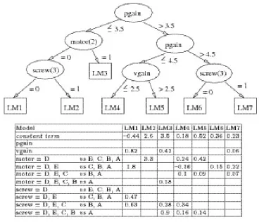
Regression trees and model trees take a common approach to addressing this problem. Their basic tree construction algorithm is as follows: branch on problem attributes in the upper part of the tree, and end with a constant or linear regression formula at the leaves. Branching points in the upper tree are chosen to maximize the reduction in standard deviation among solutions on the two sides of the split. In other words, cases with similar solutions end up on the same branch. After a certain number of branching points have been created, the remaining cases’ solutions on any branch will all be quite similar. This is the stage at which regression trees and model trees differ. Regression trees end with a leaf node that contains the mean solution for the remaining cases. Model trees end with a leaf node containing a linear model in the remaining attributes for the remaining cases’ solutions. Figure 2.5 shows an example of a model tree for the Servo dataset, one of those used in experiments in Chapter 7.
Figure 2.5: Model tree and linear models for the Servo dataset (from [Wang and Witten 1997])
[image:29.595.133.502.334.650.2]domain is partitioned into different regions, each represented by a linear model—this allows the technique to be used in domains that are not globally linear. Model trees can be thought of as an eager version of LWLR, where linear models are created based on the characteristics of the training data rather than those of the query. Chapter 7 uses the M5′ implementation of model trees [Witten and Frank 2000, pp. 201–208].
2.6 Summary
This chapter looked at some standard approaches to predicting the value of a numeric variable (i.e., regression):
Linear Regression: A single linear model is fitted to a set of numeric data points and used to predict solutions for new instances.
k-NN: For each new data instance, a number of similar stored instances are retrieved and their solutions averaged to make a prediction.
LWLR: A combination of linear regression and k-NN. For each new data instance, a local linear model is constructed from a set of similar instances and used to make a prediction.
Chapter 3
Case-Based Reasoning
The goal of this research is to construct an effective regression system using case-based reasoning (CBR). As a technology, CBR is a relatively recent invention. As a means of solving problems, however, it is among the oldest and most intuitive types of reasoning. The basic underlying idea is simple: given a new problem to solve, find a similar problem that was solved in the past and reuse its solution. Many researchers have explored this from a cognitive science perspective, and have argued that it constitutes a plausible model of the human reasoning process [Schank 1982; Kolodner 1993]. Most people solve new problems by
remembering similar problems from the past and then re-applying an old solution that meets current needs (perhaps with some alteration). The importance of prior examples has been demonstrated in all domains of human reasoning from the simplest to the most sophisticated, including mathematics [Faries and Schlossberg 1994] and medicine [Schmidt et al. 1990].
Early research into CBR arose out of a desire to represent this reasoning process in a computer model. The cognitive roots of CBR were explored at Yale University by Roger Schank and his colleagues [Schank and Abelson 1977; Riesbeck and Schank 1989]. Researchers in the AI community built on this research to develop CBR as a practical problem solving methodology (e.g., [Aamodt and Plaza 1994]). CBR has been implemented in a multitude of different systems with an enormous variety of system tasks and technologies. Underlying all of them is the simple idea of directly reusing past experiences to solve new problems. The effectiveness of this approach is based on the idea that ‘similar problems have similar solutions’ [Leake 1996]. As discussed in Section 2.2, this has been called the similarity assumption and is equivalent to saying that the world is regular. In the context of numerical regression domains that are the target of this research, it means that domains are assumed to be continuous and not overly non-linear in local regions. This assumption constitutes the
Simplicity is only one of several advantages that have contributed to CBR’s popularity over the past twenty-five years, and a number of others are presented in the following section. The new regression algorithms presented in Chapters 4 and 5 benefit from these advantages and are implemented as pure CBR systems.
3.1 Advantages of CBR
CBR’s advantages over alternative AI problem solving techniques can be summed up as follows:
CBR systems are easier to construct and maintain, and offer improved performance during operation.
These two aspects of CBR systems are discussed below.
3.1.1 Simpler system construction and maintenance
Traditional problem solving systems in AI have relied on the presence of explicit, domain dependent knowledge that is acted upon by a separate reasoning element. This broad architecture for intelligent systems is among those proposed in [Turing 1950], and systems built along these lines are known as knowledge-based systems [Aamodt 1993]. The importance of specific domain knowledge, often explicitly represented in symbolic form, is encapsulated in the ‘Knowledge Principle’:
A system exhibits intelligent understanding and action at a high level of competence primarily because of the specific knowledge that it can bring to bear: the concepts, facts, representations, methods, models, metaphors, and heuristics about its domain of endeavour. [Lenat and Feigenbaum 1991]
machine-readable format (e.g., a PROLOG rule-base). This process is fraught with difficulties, among them the following:
Is the system’s level of knowledge adequate to allow it to perform its task to the standard required? And how can this question be answered satisfactorily?
Is the knowledge accurate and consistent? Domain experts may make erroneous and contradictory statements, and mistakes can occur during both stages of the knowledge transformation process. Again, ascertaining the answer to this question is problematic because domain experts are often not qualified to inspect or edit the knowledge in its machine-readable form.
Can an expert’s experiences be conveniently represented in an explicit form such as a set of rules? Doctors, for example, rely on their many years’ experience when making decisions and often cannot list all the factors involved or the precise reasoning process followed. ‘Instinct’, ‘intuition’, ‘gut feeling’—these may play a crucial part in distinguishing expert from non-expert levels of decision making, yet representing them explicitly may be difficult or impossible.
Once knowledge has been acquired and the system constructed, how easy is it to maintain? All real-world computer systems must be continuously updated or become obsolete [Lehman 1985]. In a knowledge-based system, faulty or out-of-date knowledge must be removed and new knowledge added on an ongoing basis. Does this require regular iterations of the knowledge acquisition process, with knowledge engineers and domain experts performing a full audit of the system’s knowledge store? Such an onerous maintenance process would not be viable for most decision-support systems.
Summing up, then, knowledge elicitation is a difficult and uncertain process for knowledge-based systems (see [Forsythe and Buchanan 1989] for further discussion on this topic). Perhaps the chief advantage of CBR is that it can ease both the acquisition and maintenance of domain knowledge.
knowledge is available only in natural language); second, CBR systems need additional retrieval and adaptation knowledge to operate successfully (see Section 3.3). Even taking these into account, however, CBR’s approach to storing knowledge in cases often simplifies knowledge acquisition considerably.
Knowledge maintenance during system operation: Most knowledge in a CBR system is contained in the set of prior cases stored together in a case base (CB), where each case contains details of a single past problem and its solution. It is a straightforward matter for a domain expert to examine such a case and determine whether the problem description is inconsistent or the solution inappropriate. This accessibility allows users of a CBR system to remove faulty cases and add new ones without the aid of a knowledge engineer. This not only makes routine maintenance much easier, but also allows systems to be deployed with a minimal set of initial seed cases; additional cases can then be added by users as they become available. Note that routine removal of obsolete cases and addition of new ones allow CBR systems to adapt naturally in the presence of concept drift, a characteristic of some domains whereby the types of cases encountered changes over time [Widmer and Kubat 1996]. One domain subject to concept drift for which CBR is a natural fit is the filtering of spam email [Cunningham et al. 2003a].
3.1.2 Improved performance during operation
Ease of construction and maintenance are excellent characteristics for any AI system, but problem solving abilities are at least as important. After all, the simplest system to deploy and maintain will be useless if it offers poor performance in operation. Three criteria can be used to judge the quality of the solution offered by an AI system in response to a problem:
1. How close is the solution to the optimal solution that would be found by a committee of domain experts, or by a computer system that performed an exhaustive search? 2. How efficiently is the solution found? The level of efficiency required will vary with
the application domain. For example, a helpdesk operator may need a response within a few seconds, whereas a computer chip designer may be prepared to wait overnight for a better response according to criterion 1.
to human users, and if their conclusions are not trusted, they will (not unreasonably) be ignored. Trust may be established in two ways:
The process by which a solution is found can be laid bare to allow the user to verify that the reasoning process is sound;
Alternatively, a reasonable explanation or justification for a solution can be presented to the user.
The first approach is taken by expert systems that present users with the rules used to solve a problem. The chain of reasoning used is not always convincing (or even comprehensible) to the user, however [Moore 1994, p. 31; Barlizay et al. 1998]. The second approach may be taken if the problem-solver uses a reasoning process that is simply not accessible to humans (e.g., an artificial neural network). Once the solution has been arrived at, a second process is initiated to find an explanation that convinces the user that it is correct. This explanation may be presented as a set of rules, for example [Andrews et al. 1995].
The nature of CBR allows it to perform well according to all three of these performance criteria:
High quality solutions: In certain domains, reasoning from cases offers a distinct advantage over more abstract reasoning. It has already been pointed out that some domains may be extremely difficult to model using formal knowledge representations such as rule-sets. Domains in which relationships between important concepts are uncertain are known as weak-theory domains [Porter 1989]. Uncertainty may be due to the fact that some parts of the domain are not observable, or because aspects of the domain change over time or in response to certain events. Examples of weak-theory domains include medicine and law. Where rules are inadequate to model complex and uncertain domains, reasoning from cases may offer better solutions than logical inference from generalized models [Porter et al. 1990]. Presented with a new problem, a CBR system will retrieve stored cases that show precisely how similar problems were solved in the past. These past solutions may be presented directly to the user, or may provide the starting point for generating a solution that more closely fits the circumstances of the new problem.
from the past. This allows CBR to be used in complex domains where finding a solution from first principles may be NP-hard, for example, solving planning problems [Spalazzi 2001] or synthesising new drugs [Craw 2001].
Convincing explanations: Any computer system not trusted by its users will almost certainly fail. CBR systems have a natural advantage in instilling trust in that they can accompany each solution with the actual past cases used to derive it. Users can verify for themselves the degree of similarity between these past cases and the current one. If they are convinced that past and current problems are similar, they are likely to accept a solution similar to and derived from the solutions to these past cases. If they do not accept that the retrieved and current problems are similar, they are free to reject the proposed solution or treat it with some caution. Either way, presenting past cases to users gives a high degree of insight into the problem solving process and allows people to decide their own level of confidence in each solution [Cunningham et al. 2003b]. This is particularly useful when the suggested solution is uncertain, perhaps because similar past cases contain contradictory solutions. In this case, the user can evaluate the available evidence and decide what to do.
Two additional aspects of presenting cases as explanations are interesting to note: Cases may be used to provide explanations for solutions found using black-box
systems such as neural networks or support vector machines [Nugent and Cunningham 2004]. CBR is then used as an explanation system rather than a problem-solver.
Cases that are most convincing to the user may not be those most similar to the new case. In classification tasks, for example, cases between the new case and the decision surface may prove most compelling [Doyle et al. 2004].
3.1.3 When to use CBR
It was mentioned in Section 2.4 that all problem-solvers have a bias that makes them more suitable for certain types of problems than others. Listing the advantages of CBR serves to highlight the characteristics of those domains where CBR can most usefully be applied:
Incomplete knowledge at time of construction, and ongoing learning required: CBR systems can be deployed with a minimal set of cases, and can learn incrementally by acquiring new cases during operation. Where a domain can be fully specified during construction, this advantage is nullified.
Users’ trust in the system is important: The ability to provide concrete examples by way of explanation may be CBR’s most significant advantage. It makes CBR particularly well-suited to tasks that require complete transparency in the reasoning process, for example, decision support systems that suggest medical diagnoses based on patients’ symptoms [Schmidt and Gierl 2001].
CBR is a flexible approach that can accommodate many different problem tasks and domains; [Bartsch-Spörl et al. 1999] and [Aamodt and Plaza 1994] survey some of them. One application that has seen extensive growth in recent years is the use of CBR in recommender systems on the World Wide Web [Lorenzi and Ricci 2005]. Typical system tasks include assisting users in their choice of books, music, flights, restaurants, etc. Conversational recommender systems use user feedback to iteratively narrow down the search for a satisfactory product. The problem domain (i.e., human users choosing goods and services) matches all of the characteristics listed above, and provides an excellent example of where CBR is most useful. It is a complex, weak-theory domain in that users’ preferences cannot be precisely modelled, and indeed may change over time. The case base can be initialized with a preliminary set of products, and updated continuously as new items are introduced and others become out of date. Finally, trust is important because users will not use a recommender system unless they believe that its suggestions are helpful and unbiased.
3.2 CBR Problem Solving Methodology
CBR solves new problems by re-using solutions from similar past cases. It takes a lazy
approach to problem solving in that it does not generalize beyond the specific cases in the CB until asked to solve a new problem (this new problem is known as a query case). In particular, CBR demonstrates the following behaviour that is characteristic of all lazy problem-solvers [Aha 1997]:
Deferred problem solving: CBR systems delay processing of their inputs (i.e., new and past cases) until a query case is received.
Temporary results are discarded: Temporary results created while solving a query case are discarded—problem solving is tailored to the individual needs of each new query. Eager systems take an alternative approach. They do not work directly with past examples to solve new problems, but instead compile these experiences into a global model during an initial training phase. Examples of eager problem-solvers include neural networks, decision trees, rule-sets, and linear regression models. Lazy and eager systems have complementary advantages and disadvantages, and many of the advantages of CBR presented in Section 3.1.2 are due to its lazy nature.
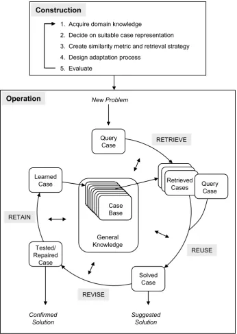
Having looked at the high-level motivations behind CBR, its advantages and appropriateness for different domains, we turn now to the mechanics of actually constructing and using a CBR system. This is fundamentally an engineering problem that can be tackled in many different ways. Based on researchers’ experience of CBR over the years, however, the process has been distilled into a series of logical steps (see Figure 3.1). These can usefully be divided into two broad phases:
Construction phase: Comprises all of the actions needed to bring a CBR system into service.
RETRIEVE
REVISE RETAIN
REUSE Query
Case
Tested/ Repaired
Case Learned
Case
New Problem
Query Case Retrieved
Cases
General Knowledge
Case Base
Confirmed
Solution Suggested Solution
1. Acquire domain knowledge
2. Decide on suitable case representation 3. Create similarity metric and retrieval strategy 4. Design adaptation process
5. Evaluate
Construction
Operation
[image:39.595.146.493.66.554.2]Solved Case
Figure 3.1: Construction and operation of a CBR system (problem solving cycle from [Aamodt and Plaza 1994])
3.2.1 Construction phase
CBR’s problem solving process was summarized above as follows: “CBR solves new problems by re-using solutions from similar past cases”. This sentence immediately suggests a number of mechanisms that must be in place before a CBR system enters operation:
Similarity metric and retrieval strategy Adaptation process
These aspects of CBR system construction are examined in the following sub-sections.
3.2.1.1 Acquisition of domain knowledge
Design of a CBR system begins with a detailed examination of the problem domain. The system task must be clearly specified and CBR’s suitability for achieving it confirmed. Domain experts may be interviewed to ascertain how problem solving was carried out in the past. Historical data based on existing, perhaps manual, systems must be collected and analysed.
We will not examine this aspect of system construction in detail, since it is common to all knowledge-based systems. The output of this phase is a clear idea of the system’s task and a rough idea of the knowledge that will be required to support it. Sufficient historical data should also have been collected to enable the assembly of an initial set of cases.
3.2.1.2 Case representation
Deciding exactly what to store in each case may involve considerable case engineering effort. Each case generally comprises two parts: a problem part containing a description of a single past problem, and a solution part containing the solution that was eventually applied. The problem part should contain all relevant information about the past situation. It should be
sufficient to enable the solution to be arrived at by a process of reasoning, so that a human expert would arrive at the same or a very similar solution. Both problem and solution parts are often represented as a set of case features or attributes, where each attribute has a particular type (e.g., numeric, string, Boolean, nominal). More complex attribute types are also possible; a quadratic-equation attribute might be represented as a set of three parameters, for example, or a graph attribute as a set of nodes and edges. ([Aha and Wettschereck 1997] describes a number of different case representation approaches.) Problem and solution attributes together constitute a case structure that is represented in software as a data structure or data type. Each case is then stored as an instance of this type.
Potential attributes are often evaluated by a process of attribute (or feature) selection [John et al. 1994] to determine which are most useful in reasoning towards the solution. Eliminating irrelevant attributes serves the dual purpose of minimizing case size and maximizing the applicability of stored cases to new problems. Note that the optimal set of attributes must be
operation). The relationship between problem attributes and the solution is one of correlation rather than causation—changes in problem attributes should correspond to changes in the solution without necessarily causing them. The hypothetical target function f that maps problem attributes ai to a solution y (i.e.,yf(a1,a2,...,an) ) is surjective because each valid set of problem attribute values maps to a single solution and different sets of attribute values can share the same solution.
Once a suitable case representation has been arrived at, the case base can be populated with an initial set of cases. These can be used as a test-set to help tune the retrieval and adaptation strategies and to confirm that they meet their performance requirements.
3.2.1.3 Similarity metric and retrieval strategy
Solving a new query begins with the retrieval of similar past cases. The retrieval process has two components: first, past cases must be assessed to determine their similarity to the query; second, similar cases must be located in a timely and efficient manner. The first component involves defining a similarity metric, that is, a function that determines the distance between any two cases. Armed with a suitable metric, a CBR system can retrieve past cases most similar to a query—these are referred to as the query’s nearest neighbours. The second component entails deciding on a suitable storage structure for the CB, and a suitable search strategy for locating cases similar to the query.
Designing a good similarity metric involves answering the following question: What does it mean to say that two cases are similar? For our purposes, the answer is that a stored case is similar to the query if its solution can easily be adapted to solve the query [Leake 1995; Bergmann et al. 2001]. Retrieving past cases based on their adaptability has been called ‘adaptation-guided retrieval’ [Smyth and Keane 1998]. The difficulty with this approach is that since the query’s solution is unknown, how can a case’s adaptability be determined without actually trying to adapt its solution and seeing how much effort is required to fit it to the query? This problem is generally resolved by recourse to the similarity assumption: similar problems are assumed to have similar solutions, and similar solutions are assumed to be easily adaptable from one to another. So cases most similar to the query are taken to be those with problem parts most similar to the query. Determining the similarity between two cases’ problem parts can be accomplished using a similarity function [Althoff and Richter 2001]. One common approach is to take the global similarity between two cases τ and ρ as the sum of the local similarities between each pair of problem attribute values:
A
a wa sim a a
Sim(τ,ρ) ( , ) (3.1)
The local similarity function sim(a,a) (also known as a comparator) can be tailored to the requirements of each individual attribute. For commonly occurring nominal and numeric attributes, the following function is often used:
continuous , nominaland , and nominal , 1 0 1 ) , ( min max a a a a a
sim a a
a a
a a a
a
(3.2)
The first part of this similarity function is used for nominal attributes in the experimental evaluation in Chapter 7. For continuous (numeric) attributes, an alternative local similarity measure is used in which Gaussian distance weighting is applied. To calculate the similarity between two attribute values, the distance between them is first normalized by converting it to a z-score (i.e., a multiple of the attribute’s standard deviation sa [Runyon and Haber 1991, p. 167]). The similarity score is then the (two-tailed) proportion of the standard normal distribution beyond this z-score:
) ,
( a a
sim proportion of standard normal distribution beyond a a a s ,
a continuous.
(3.3)
This value is most conveniently read from a lookup table rather than computed from scratch for each similarity calculation.
The second component of successful case retrieval involves designing the system in such a way that the most useful cases can be found in a timely manner. Cases may be organized with some indexing structure that enables rapid retrieval; early systems such as CYRUS [Kolodner 1983] used a structure based on Schank’s cognitively inspired dynamic memory model [Schank 1982]. More recent analysis has identified three conditions that should be met by a case retrieval mechanism [Lenz and Burkhard 1996]:
Efficiency: cases should be retrieved in a timely manner, ideally without examining every case in the CB;
Completeness: the same cases should be retrieved as would be found using an exhaustive search;
Flexibility: retrieval should be possible even when the query case is incomplete.
The case retrieval net indexing strategy was designed to meet these criteria [Lenz 1999]. It is a highly efficie