A STUDY OF THE DESIGN OF ADAPTIVE CAMBER WINGLETS
A Thesis presented to
the Faculty of California Polytechnic State University, San Luis Obispo
In Partial Fulfillment of the Requirements for the Degree Master of Science in Aerospace Engineering
by Justin Rosescu
iii
COMMITTEE MEMBERSHIP
TITLE: A Study of the Design of Adaptive Camber Winglets
AUTHOR: Justin Rosescu
DATE SUBMITTED: June 2020
COMMITTEE CHAIR: Paulo Iscold, Ph.D.
Professor of Aerospace Engineering
COMMITTEE MEMBER: David Marshall, Ph.D.
Professor of Aerospace Engineering
COMMITTEE MEMBER: Aaron Drake, Ph.D.
Professor of Aerospace Engineering
COMMITTEE MEMBER: Kurt Colvin, Ph.D.
Professor of Industrial Engineering
iv ABSTRACT
A Study of the Design of Adaptive Camber Winglets Justin Julian Rosescu
v
ACKNOWLEDGMENTS
I would like to thank all my professors for providing so much knowledge over the years. I would like to specially thank Dr. Iscold for providing deep insight and keeping me on the right track through the course of this thesis. Your timely and detailed responses to my questions were invaluable for my endeavors with this thesis, and I am honored to have worked with you.
Thank you to all my friends who have supported me throughout the years and kept me sane. All of my graduate and undergraduate friends have helped to smooth over the bumpy parts of my academic career and helped make this journey more surmountable. I would have gone crazy early in my undergraduate studies were it not for you lot, and for that I thank you.
vi
TABLE OF CONTENTS
Page
LIST OF TABLES…. ... vii
LIST OF FIGURES ... viii
NOMENCLATURE ... x
CHAPTER 1. INTRODUCTION ... 1
1.1 Effect of Winglets on Induced Drag ... 1
1.2 Effect of Winglets on Parasitic Drag ... 2
1.3 Effect of Camber ... 2
1.4 Project Objective ... 4
2. LITERATURE REVIEW ... 5
2.1 Winglet Analysis and Simulation... 5
2.2 Morphing Wing... 6
2.3 Adjustable Camber Winglets ... 7
3. METHODOLOGY ... 8
3.1 Description of Geometry ... 8
3.2 Determination of Flight Conditions ... 11
3.3 VLM Analysis ... 12
3.3.1 Calculation of Aerodynamic Forces for VLM ... 12
3.3.2 Cambered Winglet Analysis ... 16
3.3.3 Panel Method Convergence Study ... 18
3.3.4 Vortex Lattice Method Convergence Study ... 20
3.4 RANS Analysis ... 23
3.4.1 Description of RANS Geometry ... 24
3.4.2 Calculation of Aerodynamic Forces for RANS ... 25
3.4.3 RANS Flow Characteristics ... 26
3.4.4 RANS Mesh Convergence Study ... 27
3.5 Comparison of Methods ... 32
4. RESULTS ... 34
4.1 RANS Validation of VLM Results ... 34
4.1.1 Lift Validation ... 34
4.1.2 Drag Validation ... 35
4.1.2.1 Induced Drag Validation ... 35
4.1.2.2 Parasitic Drag Validation ... 35
4.1.2.3 Total Drag Validation ... 36
4.2 Winglet Camber Analysis ... 37
4.2.1 Camber Effects on Airfoil Drag ... 37
4.2.2 Camber Effects on Wing Induced Drag ... 39
4.2.3 Camber Effects on Wing Total Drag ... 39
4.3 8g Turn Efficiency ... 41
4.4 Steady Level Flight Efficiency ... 45
5. CONCLUSION ... 49
6. FUTURE WORK ... 50
REFERENCES ... 51
vii
LIST OF TABLES
Table Page
3.1 Flight Conditions for Steady Level Flight and 8g Turn ... …...…12
3.2 Continuum and Reference Settings ... 26
3.3 Mesh Settings ... 27
3.4 Total Cell Count ... 30
3.5a Domain Size Lift Comparison... 32
3.5b Domain Size Drag Comparison ... 32
viii
LIST OF FIGURES
Figure Page
1.1 Illustration of Induced Drag ... …...…2
1.2 Effect of Camber on Zero-lift Angle ... 3
1.3 Parabolic Drag Polar ... 3
1.4 Extra Edge 540 Aircraft ... 4
2.1 Effect of Winglet on Spanwise Lift Distribution ... 5
3.1a Initial Geometry with Winglets ... 9
3.1b Wing Planform View ... 9
3.1c Winglet View ... 9
3.2a Wing Airfoils ... 10
3.2b Winglet Airfoils ... 10
3.3 Vortex Lattice Model ... 11
3.4 Transition Criterion ... 14
3.5 Location of Forced Transition on the Wing ... 14
3.6 Winglet Configuration Convention ... 17
3.7 Distribution of Airfoil Panels ... 18
3.8 Panel Method Convergence Study ... 19
3.9 VLM Spanwise Wing Convergence ... 21
3.10 VLM Chordwise Wing Convergence ... 22
3.11 VLM Spanwise Winglet Convergence ... 23
3.12 RANS Domain, c = 1.6m Root Chord Length ... 25
ix
3.14 Near-wing Cell Aspect Ratio ... 28
3.15 Flow Velocity for Base Domain Size ... 29
3.16 5 m Base Size, 100-Chord Length Domain Residuals ... 31
3.17 5 m Base Size, 50-Chord Length Domain Residuals ... 32
4.1 VLM Versus RANS Lift Comparison ... 34
4.2 VLM Versus RANS Induced Drag Comparison ... 35
4.3 VLM Versus RANS Parasitic Drag Comparison ... 36
4.4 VLM Versus RANS Total Drag Comparison ... 37
4.5 Winglet Base Airfoil Parasitic Drag Polar ... 38
4.6 Winglet Top Airfoil Parasitic Drag Polar ... 38
4.7 Effect of Winglet Flap Deflection on Induced Drag ... 39
4.8 Effect of Winglet Flap Deflection on Total Drag ... 40
4.9 Effect of Winglet Flap Deflection on Efficiency ... 41
4.10 Effect of Winglet Camber at High g Turn ... 42
4.11 Effect of Winglet Flap Deflection on Lift Distribution, High g Condition ... 43
4.12 Effect of Winglet Flap Deflection on Induced Drag Distribution, High g Condition ... 43
4.13 Effect of Winglet Flap Deflection on Parasitic Drag Distribution, High g Condition ... 44
4.14 Effect of Winglet Flap Deflection on Total Drag Distribution, High g Condition ... 44
4.15 Effect of Winglet Camber at Low g Steady Level Flight ... 45
4.16 Effect of Winglet Flap Deflection on Lift Distribution, Low g Condition ... 46
4.17 Effect of Winglet Flap Deflection on Induced Drag Distribution, Low g Condition ... 46
4.18 Effect of Winglet Flap Deflection on Parasitic Drag Distribution, Low g Condition ... 47
x
NOMENCLATURE
CD Drag Coefficient
Cd Airfoil Drag Coefficient
CL Lift Coefficient
Cl Airfoil Lift Coefficient
D Drag
Di Induced Drag
E Efficiency
F Force
L Lift
N Amplification Factor Threshold
Re Reynolds Number
S Wing Area
b Wingspan
c Chord Length
g Load Factor
k, Tke Turbulent Kinetic Energy
kg Kilogram
m Meter
nf Force Direction Vector
s Second
u⸼ Freestream Velocity
v Velocity in y-direction
w Velocity in z-direction
xi
δ Percentual
ε, Tdr Turbulent Dissipation Rate
ν Kinematic Viscosity
ρ∞ Freestream Air Density
σ Boundary Layer Thickness
1 Chapter 1 INTRODUCTION
Winglets are vertical extensions attached to the wing tips of aircraft that are typically used to reduce drag at lifting conditions. This leads to an increase in span-wise efficiency compared to a wing with no winglets, but as a tradeoff, they always increase the parasitic drag of the wing. Winglets seem to be advantageous for high-lift conditions like climbing and turning, however, they may decrease efficiency for lower-lift conditions like high speed dash [1], as a result of the winglets’ separate effect on the lift-induced drag and parasitic drag of the wing.
1.1 Effect of Winglets on Induced Drag
Induced drag is the drag due to the lift generated by a finite wing. As shown in Figure 1.1, on a specific section of a finite wing at a given angle of attack, the resultant lift vector of an airfoil has a component in the freestream direction. This effect is due to the fact that a finite wing has a wingtip vortex, which induce downward momentum αi along the span, lowering the wing’s effective angle of attack αeff. Since the total lift of the wing should be measured, by definition,
2
Figure 1.1: Illustration of Induced Drag
Induced drag is proportional to the square of the lift produced by the wing. At higher lift conditions like climbing and turning, the induced drag is substantial. Winglets’ effectiveness at
reducing this induced drag is more noticeable for these conditions. However, at lower lift conditions like cruise, there is less lift being produced and therefore less induced drag, diminishing the performance gains of winglets.
1.2 Effect of Winglets on Parasitic Drag
Parasitic drag for wings refers drag due to the predominantly viscous forces, where the more surface area that is exposed to fluid flow, the more parasitic drag is produced. Since winglets increase the wetted area of wings, they will produce more parasitic drag compared to a wing without winglets. Although winglets produce slightly less induced drag at low lift conditions, this does not account for their comparatively larger increase in parasitic drag, which is why winglets are less efficient at these conditions.
1.3 Effect of Camber
3
parabolic relation with increasing angle of attack, so a cambered airfoil should be able to produce less drag for a given amount of lift since it needs a lower angle of attack to produce this lift.
Figure 1.2: Effect of Camber on Zero-lift Angle
Figure 1.3: Parabolic Drag Polar
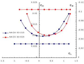
Decreasing winglet camber at high speeds should decrease the amount of lift produced by the winglet, such that it should be at minimum drag conditions and thus have the effect of minimizing drag due to the winglets. At lower speeds and higher lift conditions, increasing winglet camber should increase the lift produced by the winglet, spreading the lift distribution of the wing towards the wingtip. This enables the wing to fly at a lower angle of attack since the winglets take more of the lifting load, which should reduce the drag of the main wing.
0 0 . 0 0 5 0 . 0 1 0 . 0 1 5 0 . 0 2 0 . 0 2 5
- 1 . 5 - 1 - 0 . 5 0 0 . 5 1 1 . 5
CL
CD
- 0 . 1 2
- 0 . 1
- 0 . 0 8
- 0 . 0 6
- 0 . 0 4
- 0 . 0 2
0
CM
4
1.4 Project Objective
The objective of this thesis is to determine the effect of a variable-camber winglets on its overall efficiency, when applied to an Extra Edge 540 acrobatic race aircraft, seen in Figure 1.4 [2]. In this particular case, the goal is to minimize drag in two distinct flight conditions: i) a high lift condition based on an 8g turn at 200 knots and ii) low lift condition based on steady level flight at 200 knots. The geometry is a trapezoidal wing with winglets that were, originally, designed to minimize induced drag at high lift conditions and minimize parasitic drag at low lift conditions, and thus minimize race times for typical circuits. To achieve this goal, numerical analysis was performed on the three-dimensional CAD model of this wing. Camber changes to the winglet were made by introducing a simple plain flap at different locations along the chord of the winglet. Two numerical analysis techniques were used: i) a low-fidelity vortex lattice method (VLM) that allowed easy manipulation of winglet camber, but required separate calculation of induced and parasitic drag, and ii) a high-fidelity Reynolds Averaged Navier-Stokes method that calculated all aerodynamic forces within the same software suite but required use of computer aided design (CAD) to make camber changes.
5 Chapter 2
LITERATURE REVIEW
2.1 Winglet Analysis and Simulation
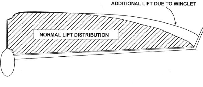
Winglet may be analyzed experimentally to obtain realistic aerodynamic forces. Through wind tunnel testing, it was discovered that winglets can provide the same increase in efficiency as horizontal wing extensions [3]. In addition, it has been shown that winglets increase the spanwise loading of an aircraft’s wing, as shown in Figure 2.1 [4]. This conclusion is the basis from which
winglets are implemented on aircraft that need an increase in efficiency for high lift conditions.
Figure 2.1: Effect of Winglet on Spanwise Lift Distribution
6
VLM is a low-fidelity method that is mainly used in preliminary design to calculate induced drag of a wing through use of integrating the radial velocity of a far-field Trefftz plane, of which the methodology will be explained in Chapter 3. It should be noted that VLM cannot calculate parasitic drag or interference drag due to complex model geometry. Other methods should be used to obtain these forces for preliminary design [6], but a more robust method like RANS that calculates all of these forces should be used to obtain accurate performance predictions [7,8].
2.2 Morphing Wing
Recently, the use of morphing wings and adaptive geometry has gained the interest of researchers as an alternative to optimize a flying vehicle for different flight conditions. Research has already been done on the feasibility of different physical actuation systems and materials by using finite element analysis and experimental testing to determine stresses seen in the physical configuration of a morphing wing or winglet [9, 10] showing promise for future implementation of these technologies in aircraft. These studies in product development enables other researchers to develop an optimal design for a wing shape based on more than one flight condition, since mechanisms for changing the shape between two or more configurations is being researched in tandem.
7
2.3 Adjustable Camber Winglets
With the research being done on creating adaptive geometry to optimize wing shapes for different flight conditions, some of these concepts carried over to determine the effect of changing the camber for winglets based on different flight conditions. However, early attempts at researching the effects of winglet camber were not promising, as researchers have found through wind tunnel experiments that any adjustment in winglet camber by using a simple plain flap at low lift flight conditions decreased efficiency over an otherwise optimized winglet [13]. The researchers admitted to limitations in their methodology as only the wing tip with winglet was tested as opposed to a full wing, so there still remains room for further analysis. A more recent study has modeled a full aircraft with adaptive camber winglets using computational fluid dynamics (CFD) and came to the same conclusion, however this study used winglet flap extensions at the trailing edge as opposed to changing the camber of a preexisting winglet [14]. While this result agrees with the notion that changing camber is detrimental to wing performance, the methodology and model setup introduced another variable in the form of winglet extension size that may adversely affect results compared to a winglet with unaltered size.
8 Chapter 3 METHODOLOGY
Two methods were used to determine the aerodynamic characteristics of winglet performance for this study. The first stage involved the use of a low-fidelity three-dimensional vortex lattice method (VLM) to determine winglet’s camber effects on lift and drag for the entire
wing. This method focused on analyzing the aerodynamic characteristics of multiple winglet camber configurations. The second method used steady Reynolds Averaged Navier-Stokes (RANS) simulations to model the air flow in a discretized domain and obtain aerodynamic forces via the pressure and shear stresses caused by the flow on the wing’s surface. Compared to VLM, RANS is more computationally expensive.
While RANS can generate a solution to the flow field over a body that is more accurate to reality than VLM, the computation time needed to simulate all the winglet configurations would significantly extend the timeline of this study [16]. If it can be proven that a lower-fidelity and computationally cheaper method like VLM can provide results as accurate as this high-fidelity computationally expensive method like RANS, then this lower-fidelity method can be used to design and analyze these winglets.
3.1 Description of Geometry
9
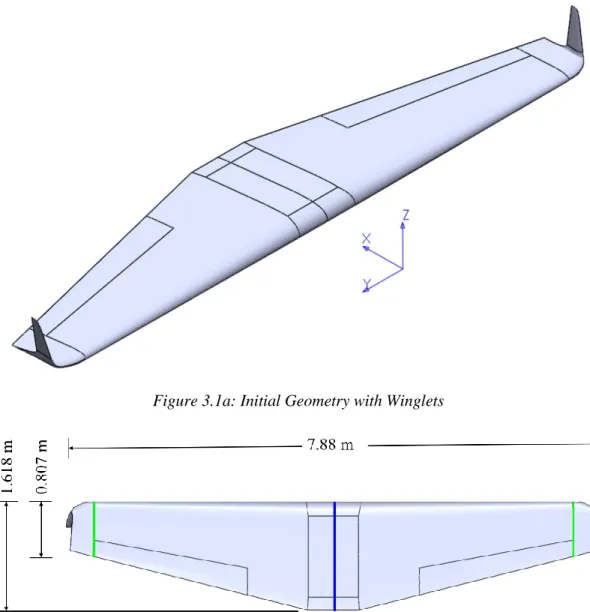
Figure 3.1a: Initial Geometry with Winglets
Figure 3.1b: Wing Planform View
10
Figure 3.2a: Wing Airfoils Figure 3.2b: Winglet Airfoils
11
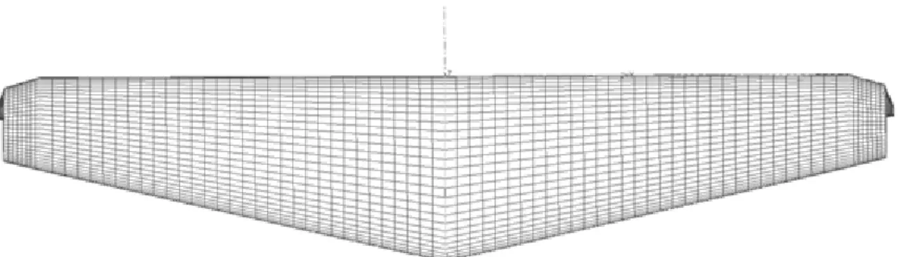
Figure 3.3: Vortex Lattice Model
3.2 Determination of Flight Conditions
For this study, lift and drag characteristics of winglet camber configurations were analyzed for different flight conditions. Winglets tend to be detrimental at lower lift conditions like steady level flight since induced drag is not significant at this flight condition; any decrease in induced drag here due to the winglets’ effect on the wingtip vortex does not account for the increase in
parasitic drag due to the wetted area of the winglets. This study aims to determine if changing winglet camber can reduce the parasitic or induced drag enough to show a noticeable decrease in total drag.
12
was needed in order to determine how much lift was necessary to produce steady level flight, and the 8g load factor for the turning condition.
Table 3.1: Flight Conditions for Steady Level Flight and 8g Turn
Steady Level Flight, 200 Knots
Airspeed 102 m/s
Mass 700 kg
Target CL 0.1191
Air Density 1.225 kg/m3 Reference Area 9.04 m2 Reference Chord 1.213 m
8g Turn, 200 Knots
Airspeed 102 m/s
Mass 700 kg
Target CL 0.9634
Air Density 1.225 kg/m3 Reference Area 9.04 m2 Reference Chord 1.213 m
For each flight condition, a target lift coefficient was used to match all winglet configurations instead of an angle of attack because changing the winglet camber alters the lift produced for a given angle of attack. This means that for a given amount a lift, the angle of attack required to produce this lift will be different based on the winglet camber. To ensure that the comparison for each winglet configuration is based on the lift required for each flight condition, lift was set to be constant and angle of attack was allowed to vary.
3.3 VLM Analysis
VLM is a method that is best suited for aerodynamic configurations that consist of thin lifting surfaces at small angles of attack [17]. This method was used to calculate lift and lift-induced drag based on the vorticity measured in the far-field Trefftz plane. Since the method only uses thin surfaces, it neglects viscous effects due to airfoil thickness. However, it is necessary to include effects of viscosity on the total forces and moments acting on a wing since total drag is the summation of viscous drag and induced drag.
3.3.1 Calculation of Aerodynamic Forces for VLM
13
XFLR5 was used to conduct batch analysis of airfoil sections that constitute the wing used in this study. XFLR5 is based on the XFOIL program, which is used to conduct two-dimensional panel method analysis. XFLR5 uses a high-order panel method combined with fully coupled viscous/inviscid interaction to obtain aerodynamic properties of airfoils at user-specified conditions. Through the interaction of incompressible potential flow and boundary layer formation equations, parasitic drag for an airfoil can be calculated. These calculations were performed for airfoils that constitute the root and tip of the wing, as well as the base and the top of the winglet [19]. For intermediate wing sections between the wing root and tip, viscous drag is interpolated based on the local wing lift [20].
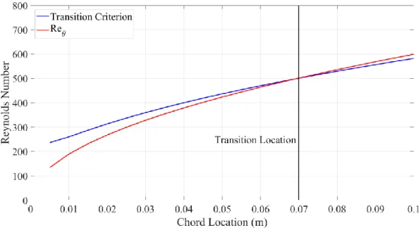
XFLR5 uses the eN method to predict boundary layer transition for steady two-dimensional flows, based on linear stability theory [21]. For this method, transition occurs when the local instability amplification rate based on velocity profile exceeds a certain threshold N, which is typically set between 7 and 9 [22]. In addition, XFLR5 allows users to set a forced transition location along the chord of an airfoil. Transition may occur when the Reynolds number based on momentum thickness exceeds the transition criterion as shown below in equations 1 and 2 [23]. For a freestream airspeed of 102 m/s, transition occurs at 0.07 m along the chord, as shown in Figure 3.4. This was set to be forced transition location for all airfoils along the span of the wing, including the winglets as shown in Figure 3.5.
Momentum Thickness: 𝜃 =0.73𝑥
√𝑅𝑒𝑥
1
Transition Criterion: 𝑅𝑒𝜃> 1.174 (1 +
22,400 𝑅𝑒𝑥
14
Figure 3.4: Transition Criterion
Figure 3.5: Location of Forced Transition on the Wing
15
It should be noted that thin airfoil theory assumes a linear relation of lift to angle of attack since this method calculates lift based on inviscid theory. As such, this method cannot accurately predict stall, which occurs at high angles of attack due to boundary layer separation. This also means that the lift produced around the stall angle cannot be accurately calculated with this method, so the accuracy results from tests at higher angles of attack are dubious.
As mentioned before, VLM uses thin airfoil theory to determine the local lift slope of airfoil sections on a wing. Thin airfoil theory assumes the lift curve slope is 2π; this is true for all airfoils
using this theory. However, increasing the airfoil’s camber lowers its zero-lift angle of attack. This means that for a given angle of attack, a cambered airfoil should produce higher lift. VLM determines the effective angle of attack for each spanwise section of the wing and relates this to each section’s individual lift curve described by its camber. Based on this, the lift for each section
can be calculated [25]. Integrating the sectional lift over the entire wingspan produces total lift for the wing, as shown in equation 3. L represents total lift and L’ is the lift due to each wing section based on its spanwise position on the wing, y.
Total Lift Calculation: 𝐿 = ∫ 𝐿′(𝑦)𝑑𝑦 𝑏 2⁄
−𝑏 2⁄
3
16 Induced Drag Calculation: 𝐷𝑖 =
1
2𝜌∞∬(𝑣
2+ 𝑤2)𝑑𝑦𝑑𝑧 𝑆
4
In order to determine how much lift was needed for the high and low g conditions, the base wing with unaltered winglet camber was tested in AVL using the flight parameters from Table 3.1. The result produced an angle of attack that was necessary for the wing to produce enough lift to fly at each condition. The wing was then tested in XFLR5 to obtain the total parasitic drag for this angle of attack. This result for total parasitic drag from XFLR5 was then input into AVL to calculate the total drag for this configuration, based on the combination of the parasitic drag calculated in XFLR5 and the induced drag calculated in AVL. Every winglet camber configuration from this point on used this same method for obtaining parasitic, induced, and total drag, while making sure to match the values for required lift found here with the base wing.
3.3.2 Cambered Winglet Analysis
17
Figure 3.6: Winglet Configuration Convention
Based on initial analysis of the changes in total drag on the wing based on winglet configuration, the actual difference in drag was too small to be compared directly. To better understand the effect of winglet configuration on wing total drag, the winglet configurations were compared in terms of a percentual to the winglet with no flap deflection. Lift and drag was normalized into coefficient of lift (CL) and coefficient of drag (CD) and was dependent on the wing angle of attack and winglet configuration. Since parasitic and induced drag were calculated using separate methods, they were compared separate to each other for each winglet configuration. The other main point of comparison between the configuration is the wing efficiency, which is the ratio of the lift the wing produced divided by the drag it produced and is shown below by equation 5. Equation 6 shows the method used for obtaining the percentual in efficiency for each winglet configuration, showing the relative improvement or diminishment of efficiency for each configuration compared to the base winglet performance.
Efficiency: 𝐸 = 𝐶𝐿
𝐶𝐷
5
Efficiency Percentual: 𝛿𝐸𝑓𝑓𝑖𝑐𝑖𝑒𝑛𝑐𝑦= 100 ×
𝐸𝐶𝑎𝑚𝑏𝑒𝑟− 𝐸𝑁𝑜 𝐶𝑎𝑚𝑏𝑒𝑟
𝐸𝑁𝑜 𝐶𝑎𝑚𝑏𝑒𝑟
6
18
the two flight conditions, the 50% hinge location at +5° and -5° deflection winglet configurations were chosen because of their noticeable effect on wing efficiency and ease of convergence in VLM and the two-dimensional panel method.
3.3.3 Panel Method Convergence Study
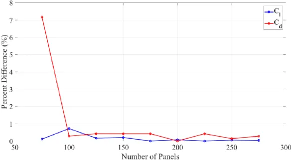
Before testing winglet camber configurations, convergence studies were conducted for the two-dimensional panel method to find the least amount of panels necessary to model the wing’s airfoils, without adversely affecting results based on numerical discretization of the airfoil. The panel method convergence study was carried out in XFLR5, using the airfoil from the root of the wing. This study was conducted at 102 m/s, which corresponds to 200 knots, the speed at which all future tests for this wing were conducted. Since the airfoil was symmetric, the angle of attack was set to 5° to provide a non-zero value for lift from which changes to lift coefficient may be observed based on total number of panels. In addition to lift, drag was also observed based on total numbers of panels. These panels were refined closer to the leading and trailing edge to better resolve the curvature and pressure distribution over these areas, as shown in Figure 3.7. The trailing edge was extended to produce a sharp point to satisfy the Kutta condition for the panel method [26].
19
For convergence studies, the equations 7 and 8 were used for calculating the percentual for lift and drag based on increasing levels of refinement. Since there is no base set of data from which to calculate deviation for this airfoil, the percent difference for each refinement level was calculated based on their deviation from the previous total panel amount: Cl current and Cd current refers to the lift and drag for the current level of refinement being analyzed and Cl previous and Cd previous refer to the lift and drag from the previous level of refinement. The condition for convergence was a total panel amount that produced minimal change compared to its preceding panel amount.
Lift Coefficient Percentual: 𝛿𝐶 𝑙= |100 ×
𝐶𝑙𝑐𝑢𝑟𝑟𝑒𝑛𝑡− 𝐶𝑙𝑝𝑟𝑒𝑣𝑖𝑜𝑢𝑠
𝐶𝑙𝑝𝑟𝑒𝑣𝑖𝑜𝑢𝑠 | 7
Drag Coefficient Percentual: 𝛿𝐶 𝑑 = |100 ×
𝐶𝑑𝑐𝑢𝑟𝑟𝑒𝑛𝑡− 𝐶𝑑𝑝𝑟𝑒𝑣𝑖𝑜𝑢𝑠
𝐶𝑑𝑝𝑟𝑒𝑣𝑖𝑜𝑢𝑠 | 8
Figure 3.8 shows the results for airfoil Cl versus number of panels, where the refinement level showed the same variation in Cl and Cd past 125 panels. This means that using any more than 125 panels for the airfoil will not significantly reduce the difference in the aerodynamic forces calculated by this method due to panel resolution. As such, 125 panels may be used for this study.
20
3.3.4 Vortex Lattice Method Convergence Study
Since VLM models a wing with horseshoe vortex strips in three-dimensional space, a different discretization method than what was used in the two-dimensional panel method needed to be used. For the main wing used in this study, only the wing root and tip locations, size, and airfoil shape were defined. Between these sections, AVL interpolated intermediate wing sections and their airfoil camber. The user determines the total number of interpolated sections and their distribution scheme between each defined wing section, as well as the total number of chordwise vortex strips and their distribution.
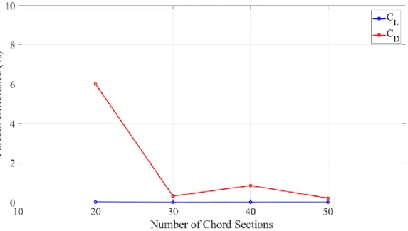
The spanwise distribution for this study was conducted first and used the same speed and angle of attack as the panel method. Spanwise sections were defined for a half-span of the wing, such that the total number of sections that were used to model the wing were double the amount listed here since the wing needed to be mirrored at the root to produce a full span. To ensure consistency with the results, the number of chordwise vortices was set to 50, which was the maximum number of chordwise points allowed by AVL. Like the panel method convergence study, relative changes in lift and drag for the entire wing was compared between the total number of wing sections, where the least amount of change between 2 sequential settings determined convergence.
21
drag was calculated, leading to variations in drag. As such, it was necessary to avoid a total number of wing sections that produce too small of a spacing between sections, so 32 wing sections were chosen as a compromise between obtaining accurate lift calculations and avoiding small spacings that can affect drag calculations.
Figure 3.9: VLM Spanwise Wing Convergence
22
Figure 3.10: VLM Chordwise Wing Convergence
23
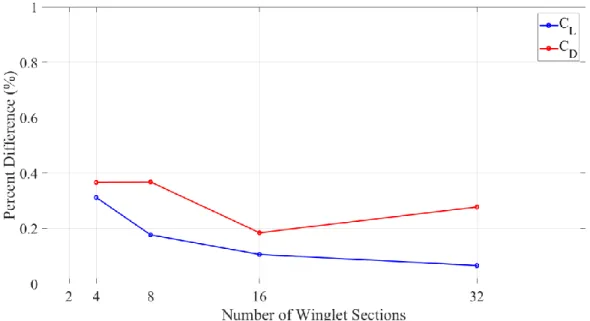
problematic sections. As long as the final number of winglet sections was between 8 and 16, the error due to winglet discretization should remain below 0.4%. For this wing setup, 10 winglet sections were the maximum number that allowed for convergence at all angles of attack tested.
Figure 3.11: VLM Spanwise Winglet Convergence
In summary, 200 panels were used to model all airfoils for two-dimensional aerodynamic analysis in XFLR5. The VLM model consisted of 32 wing sections and 10 winglet sections, with each section having 30 chordwise points.
3.4 RANS Analysis
24
for these simulations was Simcenter STAR CCM+, a computational fluid dynamics software owned by Siemens Industry Software Inc.
3.4.1 Description of RANS Geometry
Models in RANS simulations are simplified in order to resolve the airflow around a wing in a reasonable amount of time. The model used in these RANS simulations maintains the simplified trapezoidal wingspan as seen in the VLM results to maintain consistency between major model components. However, the wingtips in the RANS model must include smooth transitions between wing sections since sharp chord breaks may have adverse effects on the flow field. Therefore, this geometry should mimic what the wing would look like in reality, and thus produce similar results to the actual wing. For these simulations, all parts of the wing were modeled as no-slip walls, which allowed a boundary layer to form on the surface of the wing and enabled calculation of shear stresses tangential to the wing surface.
25
Figure 3.12: RANS Domain, c = 1.6m Root Chord Length
3.4.2 Calculation of Aerodynamic Forces for RANS
Equation 9 shows how aerodynamic forces in RANS are calculated based on the pressure and shear stresses acting on a body in the flow field [27]. f refers to a surface immersed in a flow field and nf is a user-specified direction vector. If nf is specified along the axis of freestream flow, then total drag will be calculated. Likewise, if nf is specified perpendicular to the freestream, lift will be calculated.
RANS Force Calculation: 𝐹 = ∑(𝐹𝑓
𝑝𝑟𝑒𝑠𝑠𝑢𝑟𝑒+ 𝐹
𝑓𝑠ℎ𝑒𝑎𝑟) ∙ 𝑛𝑓 𝑓
9
26
induced drag calculated by wake integration from the total drag calculated by surface pressure and shear stresses.
Figure 3.13: RANS Induced Drag Versus Trefftz Plane Location
3.4.3 RANS Flow Characteristics
Table 3.2 shows the continuum and reference values used in the simulation, which reflect the flow conditions used in the VLM simulations to maintain consistency between these two methods. The Realizable k-Ɛ turbulence model was used for its robustness and ease of convergence compared to other turbulence models
Table 3.2: Continuum and Reference Settings
Field: Value:
Freestream Velocity 102 m/s
Air Density 1.225 kg/m3
Air Kinematic Viscosity 1.855e-5 Pa-s Turbulence Model Realizable k-Ɛ Reference Area 4.52 m2
Reference Chord 1.61 m
27
3.4.4 RANS Mesh Convergence Study
RANS simulations operate by discretizing a fluid domain into finite-volume cells, from which fluid properties like velocity and pressure are calculated. Sufficiently modelling a geometry in a fluid flow may require millions of cells from which millions of calculations are made, requiring significantly more processing power than VLM or other lower-fidelity methods. In order to minimize the processing power required to simulate the flow and therefore reduce run times, a mesh refinement study must be conducted to determine the smallest mesh size that produces the most accurate results. A grid-independence study was conducted in parallel to the domain size study to determine the effect of core mesh cell size on the convergence of the simulations, and additional levels of refinement were added later for cases where a simulation initially diverged with the base settings.
Table 3.3 lists the mesh settings held constant throughout the domain study. Base size of the cells was initially set to 5 meters and was used to model the far field domain cells that would not be experiencing any flow effects from the wing. On the wing and winglet, the target size was set to 0.1% of the base size and the surface curvature was set to 720 points per circle: to allow accurate modelling of the curvature of the wing while maintaining consistent cell aspect ratio. The domain target size was set to 1,000% of base in order to enforce larger cells at the domain boundaries and reduce the total number of cells in the domain; since these areas are so far away from the wing, they should be seeing minimal effects and thus do not need a fine mesh to resolve the flow.
Table 3.3: Mesh Settings
Field: Value:
Base Size 5 m
Surface Curvature 720 points/circle Prism Layer Total Thickness 0.03 m
First-cell Height 4.103e-6 m Total Number of Prism Layers 20
Wing Target Size 0.1%
28
Figure 3.14 shows the aspect ratio of the base mesh near the wing. The reason the wing surface has low aspect ratio is because the prism layer first cell height is 4.0e-6 meters, compared to its width of 5.0e-3 meters. This is acceptable because the wall velocity for viscous flow is 0 m/s, which means that there is no flow movement that needs to be resolved on the wing surface. There is very little change in the boundary layer velocity profile along the chord or span of an object, which means that cells in the boundary layer can be much wider and longer than they are tall. However, the boundary layer velocity profile changes significantly normal to a surface in the flow field and requires the nondimensional wall y+ as described by equation 10 to be between 1 and 3 to capture this gradient accurately, using the k-Ɛ turbulence model. For the flow velocity and kinematic viscosity used in these simulations, a first-cell height of 4.0e-6 produces a wall y+ of 1. The total boundary layer height for the longest chord length in these flow conditions was calculated using equation 11 and found to be 0.024 meters, so the total prism layer height was set to be 3.0e-3 meters in order to resolve a smooth transition between the boundary layer and freestream. 20 prism layers were used to resolve the boundary layer velocity profile with the distribution being automatically determined by STAR CCM+ based on the first-cell height and the prism layer total thickness.
29
Wall y+: 𝑦+=𝑢∗𝑦
𝜈 10
Boundary Layer Height: 𝜎 = 0.37𝑥/𝑅𝑒𝑥1/5 11
Initially, the domain was arbitrarily extended 100 chord lengths away from the wing in all directions to minimize the influence of the flow from the wing on the boundaries of the domain. Based on the fluid velocity in the domain as seen in Figure 3.15, there were no flow effects near any of the boundaries in the domain. From here, the domain was decreased 75 chords, 50 chords, and 25 chords lengths in all directions in an attempt to decrease the total number of cells used in the simulation. In addition, the base size was varied between 10 meters, 7.5 meters, 5 meters, and 2.5 meters to determine the effect of finer and coarser base sizes on grid convergence.
Figure 3.15: Flow Velocity for Base Domain Size
30
The 2.5-meter meshes contained 28 million cells, which required more internal memory than what was available for the computer that was used to analyze these simulations. In order to obtain a finer mesh without exceeding computer memory limits, a base size of 3 meters was used in place of 2.5 meters for the different domain sizes. However, like with the 10-meter base size meshes, the turbulent dissipation rate for all of the 3-meter base size meshes diverged as well. It is uncertain why a finer mesh would diverge while a coarser mesh like the 7.5-meter and 5-meter base size meshes would converge, but this pattern was seen for all the domain sizes tested. As such, only the 7.5-meter and 5-meter base sizes were analyzed for this mesh refinement study.
Table 3.4 shows the cell count for the different domain sizes and base sizes. These values are important since they are proportional to how much memory each simulation requires, as well as the run times required to reach convergence. For a given base size, the total cell count is consistent among all domain sizes and seems to increase with decreasing domain size, which is the opposite of what is expected since smaller domains usually mean fewer cells are needed to fill in the mesh. One reason this may happen is because the automated mesh function inserted more cells between the wake refinement and the domain boundaries in order to satisfy the domain wall boundary conditions. It should be noted that the 100-chord domain size did not include wake refinement, but the total cell count should be proportional to the other domain sizes since the wake area is consistent between all domain sizes. In addition, the 5-meter base size for the 25-chord domain did not converge, so the 25-chord domain cannot be used for this study.
Table 3.4: Total Cell Count
100 Chords 75 Chords 50 Chords 25 Chords
7.5 m Base Size 3.77 million 3.88 million 4.01 million 3.99 million
5 m Base Size 7.19 million 7.96 million 7.78 million 7.79 million
31
size. While residuals by themselves are not a valid indicator of convergence, they are important for determining the accuracy of the results, where lower residuals equate to more accurate results since there is less change in the solution of the governing system of equations per iteration. Figures 3.16 and 3.17 depict the residuals for the 5-meter 100-chord domain and the 5-meter 50-chord domain. The continuity residual refers to the conservation of mass equation within the fluid domain while momentum residuals refer to the conservation of momentum equations for three-dimensional flow [28]. Tke and Tdr are the turbulence kinetic energy and dissipation rate respectively and are specific to the equations used to model turbulent flow in the k-Ɛ turbulence model. Not only are the residuals lower in the 100-chord domain, but they also have lower fluctuations compared to the 50-chord domain. Fluctuations in the residuals are usually caused by interactions with the domain boundaries, so it follows that the residuals would fluctuate less with the larger domain.
32
Figure 3.17: 5 m Base Size, 50-Chord Length Domain Residuals
There is a 2.36% difference between the highest and smallest values for lift and 3.07% difference between highest and lowest values for drag as seen in Tables 3.5a and 3.5b. This difference is caused by the lack of wake refinement for the 100-chord size domain. However, even without the wake refinement, there was less uncertainty in the residuals for the 100-chord domain, which means that adding the wake refinement to these meshes should produce results with lower residuals. As such, the 100-chord domain size with 7.5 m base size was used for all RANS simulations for this study, with additional refinement added when necessary to assist in simulation convergence, specifically around the leading edge to better resolve the wing curvature and in the wake region to better model turbulence dissipation.
Table 3.5a: Domain Size Lift Comparison
100
Chords 50 Chords 7.5 m Base
Size 6.68e-2 6.68e-2
5 m Base Size 6.77e-2 6.61e-2
Table 3.5b: Domain Size Drag Comparison
100
Chords 50 Chords 7.5 m Base
Size 9.76e-3 9.76e-3
5 m Base Size 9.47e-3 9.46e-3
3.5 Comparison of Methods
33
method, which means that it is only useful for small angles of attack that stay within the linear part of a wing’s lift curve. This means that VLM will assume a wing’s lift slope is still linear at high
angles of attack where in reality the wing would have a nonlinear lift curve. Based on Theory of Wing Sections, symmetric airfoils tend to have nonlinear lift curves at around 10° angle of attack, with stall occurring around 15° [24]. As will be discussed in the results chapter, the wing in the high-g condition produced an angle of attack 11°, meaning that it is possible that the lift curve for this wing may be nonlinear at this condition. Since VLM cannot accurately predict aerodynamic forces in the nonlinear portion of a wing’s lift slope, it was necessary to validate whether the lift
34 Chapter 4 RESULTS
4.1 RANS Validation of VLM Results
Since VLM requires two different methods to obtain induced and parasitic drag separately, it became necessary to compare these values to the total drag obtained from RANS to ensure that these two separate methods were valid. In order to compare these methods separately, the total drag in RANS was separated into induced and parasitic drag. A range of angles of attack from 0° to 10° was tested to obtain an overall view of the behavior.
4.1.1 Lift Validation
As shown in Figure 4.1, there is no discernable difference between lift calculated in VLM for all tested angles of attack. These angles of attack lie on the linear portion of the wing’s lift curve, which is why the results from VLM and RANS match. This is important because the wing needed an angle of attack of 0.65° to produce enough lift to fly at the low g flight condition, while the high g flight condition required 11° angle of attack.
35
4.1.2 Drag Validation
VLM requires separate calculation for induced and parasitic drag, whereas RANS calculated total drag as a combination of pressure and viscous forces on the wing. To determine the accuracy of induced and parasitic drag from VLM separately, the total drag calculated from RANS was divided into induced and parasitic drag then directly compared to VLM results.
4.1.2.1 Induced Drag Validation
In Figure 4.2, the induced drag in VLM and RANS follow a parabolic trend. However, VLM overpredicts induced drag above an angle of attack of 4°. This may be due to the effect of Trefftz plane placement in RANS, as the calculated induced drag decreases as Trefftz plane distance from the wing increases.
Figure 4.2: VLM Versus RANS Induced Drag Comparison
4.1.2.2 Parasitic Drag Validation
36
method is a lower order method suitable for simple two-dimensional flows but cannot be adapted to more complex three-dimensional flows [21], whereas the k-Ɛ turbulence model is more suited for complex three-dimensional flows, so long as there are no strong pressure gradients [29]. The inability for the eN transition model to calculate complex flow limits its accuracy for determining viscous forces due to turbulence, hence its underpredicting of parasitic drag compared to RANS.
Figure 4.3: VLM Versus RANS Parasitic Drag Comparison
4.1.2.3 Total Drag Validation
37
Figure 4.4: VLM Versus RANS Total Drag Comparison
4.2 Winglet Camber Analysis
With VLM validated against RANS, the next step of this study was to analyze the effect of cambered winglets on the aerodynamic forces produced by this wing. VLM allows for easy manipulation of flap hinge location and deflection, so it was used to obtain these forces. To better understand the overall effect of winglet camber changes on the aerodynamic forces produced by the entire wing, the behavior for winglets with a hinge at 50% chord and deflected +5° and -5° was compared to a winglet with no flap deflection for a range of angles of attack and CL. The low g steady level flight at 200 knots CL of 0.1191 and the high 8g turn at 200 knots CL of 0.9634 are denoted in the following figures.
4.2.1 Camber Effects on Airfoil Drag
38
winglet airfoils if the effective angle of attack of these airfoils is greater than 0°. However, the effective angle of attack for these airfoils at the low g condition is around -2°, where a negative flap deflection increases the parasitic drag compared to no flap deflection. Conversely, a positive flap deflection results in less parasitic drag for this condition.
Figure 4.5: Winglet Base Airfoil Parasitic Drag Polar
39
4.2.2 Camber Effects on Wing Induced Drag
The effect of flap deflection on induced drag for the entire wing was less pronounced than their effect on parasitic drag, so the induced drag for winglet configurations were compared against the winglets with no camber as a percentual, as shown in Figure 4.7. The positive winglet flap deflection produced a 20% increase in induced drag for the low g flight condition over a winglet with no flap deflection. However, the induced drag at the high g flight condition shows a 1% decrease in induced drag, meaning that the winglet with +5° of flap deflection is more efficient at this condition than the winglet with no flap deflection. The -5° winglet deflection produced 10% increase in induced drag at the low lift condition, while at the high g condition, the negative flap deflection produced a 1.3% increase in drag.
Figure 4.7: Effect of Winglet Flap Deflection on Induced Drag
4.2.3 Camber Effects on Wing Total Drag
40
in drag for most of the range of lift compared to no flap deflection. The discrepancy between the 1% decrease in induced drag and 0.65% decrease in total drag for the +5° flap deflection at the high g condition comes from the increase in parasitic drag at this condition, however the reduction in induced drag was enough to provide a net benefit for this configuration. The effect of the winglet flap deflections on efficiency is shown in Figure 4.9, where no flap deflection produced the highest efficiency for the low g condition and +5° flap deflection produced the highest efficiency for the high g condition.
41
Figure 4.9: Effect of Winglet Flap Deflection on Efficiency
4.3 8g Turn Efficiency
42
Figure 4.10: Effect of Winglet Camber at High g Turn
A detailed investigation of the winglets’ effect on the entire wing’s lift and drag
distribution was carried out on the 50% chord hinge location for the +5° and -5° flap deflections to explain why positive flap deflections may benefit efficiency at high g conditions over negative or no flap deflection. Based on the wing’s lift distribution as seen in Figure 4.11, the positive
winglet deflection provides more lift towards the end of the winglet as opposed to the other configurations, up to 4% near the end of the span. This is accompanied by an increase in induced drag towards the wing tip, but less induced drag in the main span of the wing for this
43
Figure 4.11: Effect of Winglet Flap Deflection on Lift Distribution, High g Condition
Figure 4.12: Effect of Winglet Flap Deflection on Induced Drag Distribution, High g Condition
44
Figure 4.13: Effect of Winglet Flap Deflection on Parasitic Drag Distribution, High g Condition
Figure 4.14: Effect of Winglet Flap Deflection on Total Drag Distribution, High g Condition
45
difference for an air race where a fraction of a second can determine whether an aircraft wins or loses the race.
4.4 Steady Level Flight Efficiency
The percentual differences for different winglet configurations for the low g condition is shown in Figure 4.15. An important note is that adding any winglet reduces the wing efficiency compared to a wing with no winglet due to the additional parasitic drag caused by the increased wetted area of the winglet and the low importance of induced drag for this flight condition. Deflecting the winglet flap by any amount in either direction decreased wing efficiency compared to a winglet with no flap deflection and moving the flap hinge towards the leading edge of the winglet amplifies the flap’s effect on efficiency.
Figure 4.15: Effect of Winglet Camber at Low g Steady Level Flight
46
flap deflections decrease the loading and the induced drag of the winglets. It should be noted that any winglet deflection does not produce a noticeable change in lift or induced drag for the main span of the wing compared to winglet loading.
Figure 4.16: Effect of Winglet Flap Deflection on Lift Distribution, Low g Condition
Figure 4.17: Effect of Winglet Flap Deflection on Induced Drag Distribution, Low g Condition
47
in airfoil curvature caused by the hinge and flap deflection causes an increase in parasitic drag for any deflection, with negative deflections causing a larger increase in drag than positive deflections. It can be seen that at the base and top of the winglet, the +5° flap deflection produces less parasitic drag than the winglet with no flap deflection, as referenced earlier by Figures 4.5 and 4.6. However, this deflection still produces more parasitic drag over the rest of the winglet span. This increase in parasitic drag for both positive and negative deflections is much larger in magnitude than induced drag and causes the total drag to increase over the winglet with no deflections, as shown in Figure 4.19.
48
Figure 4.19: Effect of Winglet Flap Deflection on Total Drag Distribution, Low g Condition
49 Chapter 5 CONCLUSION
A numerical study of the effect of changing winglet camber on the efficiency for an acrobatic race plane wing was performed using a low-fidelity vortex lattice method. This method was validated against a high-fidelity Reynolds Averaged Navier-Stokes computational fluid dynamics method to determine where the limitations of VLM prevented computation of accurate results. It was found that VLM can produce accurate results for lower lift conditions, but the drag results of VLM increasingly diverged from RANS drag calculations with increasing CL. However, VLM can be used to quickly test many configurations and optimize a winglet design, from which a wind tunnel model or flight test apparatus can be built to obtain values for efficiency that more reflect the flight conditions seen in reality.
Based on VLM results of the two flight regimes tested, a low g steady level flight condition at 200 knots and an 8g turn at 200 knots, it was shown that positive winglet flap deflections can increase the wing efficiency at the high g condition. For the low g flight condition, it was determined that any deflection in the winglet flap produced more drag, and thus decrease efficiency. Therefore, the most efficient winglet configuration would be the winglet with no flap deflection for this high-speed condition.
50 Chapter 6 FUTURE WORK
Since the increase in parasitic drag due to the plain flap deflection decreased efficiency for the high speed condition, it is of interest to perform the same analysis on the same wing used in this study, but for a flap with no discontinuity in winglet camber curvature. A study using a smooth transition in camber curvature for the winglet would determine if a more complex change in geometry can produce higher efficiencies for this high-speed condition.
Due to the lack of agreement between RANS and VLM drag results for the high g condition, wind tunnel or flight testing should be performed with this adaptive camber winglet at this condition to provide another source of validation, where the results will determine which of the two numerical methods used in this study is more accurate to reality.
Numerical analysis for adaptive camber winglets on a fully modelled aircraft should be attempted to determine the winglets’ effect on aircraft efficiency and interaction with the entire
body of the aircraft. The ability for VLM to model an aircraft fuselage is limited [17], but RANS or other high-fidelity methods involving domain discretization like large eddy simulation or direct numerical simulation can be used to model and analyze complex geometry.
51 REFERENCES
[1] Whitcomb, Richard T., “A Design Approach and Selected Wind-Tunnel Results at High
Subsonic Speeds for Wing-tip Mounted Winglets,” NASA Technical Note D-8260, July 1976
[2] Daily News Hungary, https://dailynewshungary.com/red-bull-air-race-2017-results-photos/ [3] Jones, R. T., Lasinki, T. A., “Effect of Winglets on the Induced Drag of Ideal Wing Shapes,”
NASA Technical Memorandum 81230, Sept. 1980
[4] Colling, J., “Sailplane Glide Performance and Control Using Fixed and Articulating Winglets,” NASA CR-198579, May 1995
[5] Rademacher, P. R., “Winglet Performance Evaluation through the Vortex Lattice Method,”
Embry-Riddle Aeronautical University Scholarly Commons, May 2014
[6] Chattot, Jean-Jacques, “Low Speed Design and Analysis of Wing/Winglet Combinations Including Viscous Effects,” Journal of Aircraft, Vol. 43, No. 2, April 2006
[7] Maughmer, M. D., “The Design of Winglets for High-performance Sailplanes,” AIAA Paper 2001-2406, 2001
[8] Azlin, M. A et al., “CFD Analysis of Winglets at Low Subsonic Flow,” Proceedings of the
World Congress on Engineering, Vol I, July 2011.
[9] Ursache, Narcis M. et al., “Technology Integration for Active Poly-Morphing Winglets Development,” Proceedings of SMASIS 2008, October 2008
[10] Wang, Chen et al., “Investigating the Benefits of Morphin Wing Tip Devices – A Case Study,” International Forum on Aeroelasticity and Structural Dynamics, June 2015 [11] Vos, R., Gürdal, Z., Abdalla, M., “Mechanism for Warp-Controlled Twist of a Morphing
52
[12] De Breuker, R. V. R, Barrett, R., Tiso, P., “Morphing Wing Flight Control via Post-Buckled Precompressed Piezoelectric Actuators,” Journal of Aircraft, Vol. 44, No. 4, Jul. 2007,
pp. 1060-1068, doi: 10.2514/1.21292
[13] Lyu, Z., Martins, J. R. R. A., “Aerodynamic Shape Optimization of an Adaptive Morphing Trailing-Edge Wing,” Journal of Aircraft, Vol. 52, No. 6, Nov. 2015, pp. 1951-1970, doi: 10.2514/1.C033116
[14] Park, P. S., Rokhsaz, K., “Effects of a Winglet Rudder on Lift-to-Drag Ratio and Wake Vortex Frequency,” AIAA Paper 2003-4069, June 2003
[15] Eguea, João Paulo et al., “Study on a Camber Adaptive Winglet,” Applied Aerodynamics Conference, AIAA, Atlanta, Georgia, June 2018, doi: 10.2514/6.2018-3960
[16] Singh, Diwakar et al., “A Multi-Fidelity Approach for Aerodynamic Performance Computations of Formation Flight,” MDPI, June 2018
[17] Drela, M., Youngren, H., “AVL 3.36 User Primer,” Feb. 2017
[18] Hough, Gary R., “Lattice Arrangements for Rapid Convergence,” Vortex Lattice Utilization, NASA SP-405, May 1976
[19] Drela, M., Youngren, H., “XFOIL 6.9 User Primer,” Nov. 2001
[20] Deperrois, André, “Theoretical Limitations and Shortcomings of XFLR5,” June 2019
[21] van Ingen, J.L., “The eN method for transition prediction. Historical review of work at TU Delft,” AIAA Paper 2008-3830, June 2008
[22] Kaynak, Unver et al., “Transition Modeling for Low to High Speed Boundary Layer Flows with CFD Applications,” intechopen, Jan. 2019, doi: 10.5772/intechopen.83520
[23] Moran, Jack, “An Introduction to Theoretical and Computational Aerodynamics,” John
Wiley & Sons, 1984, ISBN: 0-471-47491-4
53
[25] Monsch, Scott, “A Study of Induced Drag and Spanwise Lift Distribution for
Three-Dimensional Inviscid Flow Over a Wing,” Engineering Mechanics Commons, May 2007
[26] Anderson, John D., “Fundamentals of Aerodynamics,” Fifth Edition, McGraw-Hill, 2010, ISBN: 978-0-07-339810-5
[27] Siemens, “Force,” Star CCM+ User Guide, 2020
[28] Hall, Nancy, “Navier-Stokes Equations 3-dimensional-unsteady,” NASA, May 2015, https://www.grc.nasa.gov/www/k-12/airplane/nseqs.html
54 APPENDIX
Table A1: Airfoil Coordinates
Wing Root Wingtip Winglet Base Winglet Top
1.00000 0.00000 0.99431 0.00098 0.98567 0.00244 0.97696 0.00393 0.96818 0.00536 0.95937 0.00671 0.95046 0.00797 0.94131 0.00920 0.93188 0.01041 0.92209 0.01162 0.91195 0.01283 0.90151 0.01405 0.89082 0.01526 0.87983 0.01647 0.86845 0.01769 0.85656 0.01890 0.84412 0.02013 0.83120 0.02140 0.81787 0.02268 0.80417 0.02397 0.79018 0.02526 0.77596 0.02654 0.76154 0.02784 0.74700 0.02913 0.73236 0.03039 0.71763 0.03165 0.70285 0.03291 0.68808 0.03418 0.67332 0.03544 0.65857 0.03669 0.64379 0.03797 0.62897 0.03925 0.61410 0.04057 0.59918 0.04189 0.58424 0.04324 0.56926 0.04461 0.55425 0.04599 0.53921 0.04740 0.52417 0.04881 0.50912 0.05023 0.49406 0.05167 0.47901 0.05312 0.46397 0.05456 0.44897 0.05600
1.00000 0.00000 0.99501 0.00093 0.98713 0.00239 0.97880 0.00393 0.97004 0.00545 0.96087 0.00687 0.95131 0.00821 0.94140 0.00948 0.93119 0.01069 0.92073 0.01185 0.91003 0.01297 0.89908 0.01406 0.88788 0.01511 0.87647 0.01612 0.86491 0.01710 0.85317 0.01804 0.84127 0.01897 0.82917 0.01986 0.81683 0.02074 0.80431 0.02159 0.79163 0.02241 0.77884 0.02322 0.76600 0.02401 0.75313 0.02478 0.74028 0.02553 0.72747 0.02625 0.71473 0.02694 0.70210 0.02762 0.68967 0.02833 0.67724 0.02921 0.66459 0.03011 0.65178 0.03102 0.63887 0.03195 0.62586 0.03290 0.61277 0.03386 0.59964 0.03483 0.58649 0.03581 0.57331 0.03681 0.56013 0.03782 0.54695 0.03884 0.53378 0.03986 0.52064 0.04088 0.50755 0.04192 0.49446 0.04296
1.00000 0.00000 0.99630 0.00073 0.98978 0.00203 0.98187 0.00361 0.97277 0.00544 0.96303 0.00741 0.95306 0.00941 0.94294 0.01148 0.93276 0.01354 0.92253 0.01563 0.91228 0.01774 0.90204 0.01986 0.89180 0.02200 0.88158 0.02413 0.87151 0.02626 0.86144 0.02833 0.85130 0.03041 0.84116 0.03249 0.83104 0.03453 0.82098 0.03655 0.81097 0.03854 0.80095 0.04051 0.79086 0.04249 0.78066 0.04445 0.77041 0.04643 0.76015 0.04838 0.74991 0.05028 0.73966 0.05218 0.72941 0.05405 0.71923 0.05588 0.70913 0.05767 0.69902 0.05940 0.68892 0.06114 0.67889 0.06282 0.66883 0.06448 0.65878 0.06609 0.64876 0.06765 0.63862 0.06919 0.62847 0.07071 0.61835 0.07216 0.60820 0.07354 0.59801 0.07487 0.58781 0.07615 0.57765 0.07738
55 0.43401 0.05745
0.41912 0.05887 0.40428 0.06028 0.38954 0.06167 0.37490 0.06302 0.36039 0.06434 0.34604 0.06561 0.33185 0.06682 0.31783 0.06795 0.30400 0.06902 0.29039 0.06999 0.27699 0.07087 0.26382 0.07166 0.25093 0.07235 0.23832 0.07292 0.22604 0.07339 0.21410 0.07376 0.20255 0.07401 0.19143 0.07415 0.18073 0.07416 0.17047 0.07407 0.16069 0.07387 0.15138 0.07356 0.14252 0.07315 0.13412 0.07263 0.12618 0.07201 0.11865 0.07129 0.11153 0.07049 0.10479 0.06962 0.09842 0.06869 0.09240 0.06770 0.08670 0.06666 0.08132 0.06557 0.07623 0.06442 0.07141 0.06323 0.06684 0.06199 0.06252 0.06069 0.05842 0.05935 0.05453 0.05796 0.05084 0.05654 0.04734 0.05506 0.04402 0.05353 0.04088 0.05196 0.03789 0.05035 0.03505 0.04870 0.03237 0.04703 0.02983 0.04532 0.02742 0.04358 0.02515 0.04182 0.02299 0.04005 0.02096 0.03826
0.48138 0.04400 0.46831 0.04504 0.45523 0.04609 0.44215 0.04714 0.42910 0.04818 0.41607 0.04920 0.40304 0.05024 0.38999 0.05126 0.37698 0.05226 0.36400 0.05325 0.35107 0.05420 0.33818 0.05512 0.32534 0.05601 0.31258 0.05685 0.29990 0.05765 0.28732 0.05838 0.27480 0.05905 0.26239 0.05966 0.25008 0.06019 0.23789 0.06066 0.22583 0.06104 0.21394 0.06135 0.20225 0.06156 0.19078 0.06168 0.17957 0.06169 0.16865 0.06160 0.15806 0.06141 0.14785 0.06109 0.13802 0.06066 0.12862 0.06012 0.11967 0.05947 0.11119 0.05871 0.10317 0.05786 0.09564 0.05694 0.08858 0.05594 0.08199 0.05487 0.07584 0.05375 0.07011 0.05256 0.06477 0.05132 0.05978 0.05004 0.05514 0.04871 0.05081 0.04733 0.04678 0.04591 0.04300 0.04445 0.03948 0.04296 0.03618 0.04143 0.03310 0.03988 0.03021 0.03831 0.02752 0.03672 0.02499 0.03511 0.02263 0.03349
0.56757 0.07853 0.55746 0.07959 0.54735 0.08061 0.53732 0.08157 0.52736 0.08247 0.51725 0.08329 0.50704 0.08405 0.49678 0.08478 0.48655 0.08545 0.47638 0.08606 0.46623 0.08658 0.45593 0.08703 0.44562 0.08747 0.43548 0.08786 0.42554 0.08815 0.41558 0.08828 0.40545 0.08835 0.39523 0.08838 0.38488 0.08844 0.37461 0.08851 0.36445 0.08852 0.35455 0.08844 0.34454 0.08820 0.33436 0.08790 0.32414 0.08757 0.31401 0.08721 0.30388 0.08675 0.29368 0.08621 0.28343 0.08563 0.27327 0.08500 0.26320 0.08429 0.25310 0.08349 0.24293 0.08262 0.23285 0.08171 0.22287 0.08070 0.21287 0.07960 0.20287 0.07843 0.19297 0.07717 0.18313 0.07582 0.17327 0.07436 0.16343 0.07282 0.15379 0.07121 0.14425 0.06946 0.13471 0.06758 0.12524 0.06560 0.11596 0.06351 0.10681 0.06127 0.09776 0.05890 0.08888 0.05638 0.08014 0.05370 0.07162 0.05089
56 0.01903 0.03646
0.01721 0.03466 0.01549 0.03286 0.01387 0.03106 0.01234 0.02926 0.01091 0.02746 0.00957 0.02567 0.00831 0.02388 0.00715 0.02209 0.00607 0.02031 0.00509 0.01853 0.00419 0.01676 0.00339 0.01499 0.00266 0.01324 0.00203 0.01149 0.00148 0.00974 0.00101 0.00801 0.00063 0.00630 0.00035 0.00461 0.00014 0.00295 0.00003 0.00130 0.00000 -0.00032 0.00006 -0.00194 0.00021 -0.00357 0.00044 -0.00520 0.00075 -0.00686 0.00114 -0.00854 0.00163 -0.01025 0.00220 -0.01199 0.00286 -0.01374 0.00361 -0.01551 0.00445 -0.01729 0.00538 -0.01907 0.00639 -0.02084 0.00749 -0.02263 0.00868 -0.02441 0.00996 -0.02620 0.01133 -0.02800 0.01279 -0.02980 0.01435 -0.03160 0.01600 -0.03340 0.01775 -0.03520 0.01961 -0.03700 0.02157 -0.03880 0.02364 -0.04058 0.02583 -0.04236 0.02814 -0.04412 0.03059 -0.04585 0.03318 -0.04754 0.03591 -0.04921 0.03879 -0.05084
0.02042 0.03187 0.01834 0.03025 0.01641 0.02864 0.01460 0.02703 0.01291 0.02543 0.01133 0.02383 0.00986 0.02225 0.00850 0.02067 0.00724 0.01910 0.00608 0.01753 0.00502 0.01597 0.00407 0.01440 0.00323 0.01284 0.00248 0.01129 0.00184 0.00974 0.00129 0.00821 0.00084 0.00670 0.00049 0.00521 0.00023 0.00374 0.00007 0.00230 -0.00000 0.00088 0.00002 -0.00053 0.00014 -0.00192 0.00035 -0.00331 0.00064 -0.00470 0.00103 -0.00609 0.00150 -0.00749 0.00205 -0.00890 0.00270 -0.01033 0.00345 -0.01178 0.00429 -0.01325 0.00523 -0.01475 0.00628 -0.01628 0.00745 -0.01784 0.00873 -0.01943 0.01014 -0.02104 0.01165 -0.02266 0.01327 -0.02429 0.01501 -0.02591 0.01686 -0.02752 0.01882 -0.02913 0.02091 -0.03074 0.02314 -0.03235 0.02553 -0.03397 0.02808 -0.03558 0.03081 -0.03718 0.03373 -0.03875 0.03685 -0.04030 0.04019 -0.04181 0.04377 -0.04330 0.04759 -0.04475
0.06338 0.04795 0.05547 0.04488 0.04792 0.04167 0.04078 0.03835 0.03413 0.03497 0.02818 0.03167 0.02300 0.02849 0.01853 0.02544 0.01471 0.02261 0.01151 0.02005 0.00886 0.01775 0.00671 0.01560 0.00499 0.01358 0.00361 0.01165 0.00250 0.00984 0.00163 0.00815 0.00096 0.00660 0.00046 0.00518 0.00012 0.00387 -0.00009 0.00267 -0.00016 0.00158 -0.00010 0.00058 0.00009 -0.00034 0.00040 -0.00116 0.00084 -0.00192 0.00139 -0.00262 0.00205 -0.00326 0.00282 -0.00385 0.00372 -0.00440 0.00474 -0.00491 0.00590 -0.00538 0.00720 -0.00582 0.00868 -0.00623 0.01036 -0.00661 0.01228 -0.00697 0.01452 -0.00731 0.01718 -0.00764 0.02044 -0.00800 0.02455 -0.00845 0.02959 -0.00914 0.03508 -0.00995 0.04102 -0.01065 0.04816 -0.01126 0.05672 -0.01187 0.06580 -0.01240 0.07513 -0.01281 0.08490 -0.01308 0.09495 -0.01330 0.10494 -0.01344 0.11502 -0.01348 0.12525 -0.01347