Nestedness in networks: A theoretical model
and some applications
MichaelD. König
Department of Economics, University of Zurich
ClaudioJ. Tessone
Department of Management, Technology, and Economics, ETH Zurich
YvesZenou
Department of Economics, Stockholm University and IFN
We develop a dynamic network formation model that can explain the observed nestedness in real-world networks. Links are formed on the basis of agents’ cen-trality and have an exponentially distributed lifetime. We use stochastic stability to identify the networks to which the network formation process converges and find that they are nested split graphs. We completely determine the topological properties of the stochastically stable networks and show that they match fea-tures exhibited by real-world networks. Using four different network data sets, we empirically test our model and show that it fits well the observed networks. Keywords. Nestedness, Bonacich centrality, network formation, nested split graphs.
JELclassification. A14, C63, D85.
1. Introduction
Nestedness is an important aspect of real-world networks.1 For example, the organi-zation of the New York garment industry (Uzzi 1996) and of the Fedwire bank network
Michael D. König:[email protected] Claudio J. Tessone:[email protected]
Yves Zenou:[email protected]
We would like to thank Nicola Persico, two anonymous referees, Phillip Bonacich, Yann Bramoullé, Ulrik Brandes, Guido Caldarelli, Sanjeev Goyal, Patrick Groeber, Matt Jackson, Matteo Marsili, Fernando Vega-Redondo, Douglas White, Eric Gilson, and George Papanicolaou as well as the participants of the 2009 Dy-namics of Institutions and Markets in Europe (DIME) conference in Paris, the 2009 Trento Summer School, the 2009 Human Sciences and Complexity (HSC) conference at the University of California–San Diego, the 2009 Workshop on the Economics of Social Networks at Laval University, the Microeconomic Theory Semi-nar at University of California–Berkeley in 2009, the Theory Workshop at the Kellog School of Management (MEDS) at Northwestern University in 2010, and the 2011 Society for Advanced Economic Theory (SAET) conference in Faro for their helpful comments. We would like to thank the Austrian National Bank for pro-viding access to the data. Michael D. König acknowledges financial support from Swiss National Science Foundation through research Grant PBEZP1–131169, and thanks SIEPR and the Department of Economics at Stanford University for their hospitality during 2010–2012.
1A network exhibitsnestednessif the neighborhood of a node is contained in the neighborhoods of the
nodes with higher degrees.
Copyright©2014 Michael D. König, Claudio J. Tessone, and Yves Zenou. Licensed under theCreative Com-mons Attribution-NonCommercial License 3.0. Available athttp://econtheory.org.
(Soramaki et al. 2007) is nested in the sense that their organization is strongly hierarchi-cal. If we consider, for example, the Fedwire network, it is characterized by a relatively small number of strong flows (many transfers) between banks, with the vast majority of linkages being weak to nonexisting (few to no interbank payment flows). Further-more, the topology of this network is highlydissortative since large banks are dispro-portionately connected to small banks and vice versa; the average bank was connected to15others. In other words, most banks have only a few connections, while a small number of “hubs” have thousands.Åkerman and Larsson (forthcoming), who study the evolution of the global arms trade network using a unique data set on all international transfers of major conventional weapons over the period 1950–2007, also find that these networks are nested and dissortative in the sense that big countries mainly trade arms with small countries, but small countries do not trade with each other. Using aggregate bilateral imports from 1950 to 2000,De Benedictis and Tajoli (2011)analyze the struc-ture of the world trade network over time, detecting and interpreting patterns of trade ties among countries. Figure 3 in their paper shows a clearcore–periphery structure, in-dicating nestedness of their networks. Interestingly, in all these networks, dissortativity arises naturally since “big” agents tend to interact with “small” agents and vice versa. For example, banks seek relationships with each other that are mutually beneficial. As a result, small banks interact with large banks for security, lower liquidity risk, and lower servicing costs, and large banks may interact with small banks in part because they can extract a higher premium for services and can accommodate more risk.
Surprisingly, nestedness has not been studied from a theoretical point of view, even though other salient features of networks such as “small world” properties with high clustering and short average path lengths (Watts and Strogatz 1998) as well as “scale-free” or power-law degree distributions (Barabási and Albert 1999) have received a lot of attention.2
The first aim of this paper is to propose a dynamic network formation model that exhibits not only the standard features of real-world networks (small worlds, high clus-tering, short path lengths, and a power-law degree distributions), but alsonestedness
and dissortativity. The second aim is to provide a microfoundation for the network formation process where linking decisions are based on the utility maximization of each agent rather than on a random process, which is often assumed in most dy-namic models of network formation. The last aim of this paper is to provide some evidence that our model matches well some real-world network features (interbank loans, trade in conventional goods, and arms trade between countries), especially their nestedness.
To be more precise, we develop a dynamic model where, at each period of time, agents play a two-stage game: in the first stage, as inBallester et al. (2006), agents play their equilibrium contributions proportional to theirBonacich centrality,3while in the
2SeeJackson and Rogers (2007), who propose a model that has all these features, but not nestedness. 3Centrality is a fundamental measure of the importance of actors in social networks. SeeWasserman and Faust (1994)for an introduction and survey. The Bonacich centrality, introduced byBonacich (1987), of a particular node counts the total number of paths that start from this node in the graph, weighted by a decay factor based on path length.
second stage, a randomly chosen agent can update her linking strategy by creating a new link as a best response to the current network. Links do not last forever, but have an exponentially distributed lifetime. The most valuable links (i.e., the ones with the highest Bonacich centrality) decay at a lower rate than those that are less valuable. As a result, the formation of social networks can be regarded as a tension between the search for new linking opportunities and the volatility that leads to the decay of existing links.
We introduce noise into the decision process to form links (see, e.g.,Sandholm 2010), and analyze the limit of the invariant distribution, thestochastically stablenetworks, as the noise vanishes to zero.4We first show that in this limit, starting from arbitrary initial conditions, at each period of time, the network generated by this dynamic process is a
nested split graph. These graphs, which are relatively well known in the applied mathe-matics literature (Cvetkovi´c and Rowlinson 1990,Mahadev and Peled 1995), have a very nice and simple structure that make them very tractable. To the best of our knowledge, this is the first time that a complex dynamic network formation model can be charac-terized by such a simple structure in terms of networks it generates. By doing so, we are able to bridge the economics literature and the applied mathematics/physics literatures in a simple way. Because of their simple features, we then show that degree, closeness, eigenvector, and Bonacich centrality induce the same ordering of nodes in a nested split graph (this is also true for betweenness centrality if the ordering is not strict). This im-plies, in particular, that if we had a game where agents formed links according to mea-sures of centrality (such as degree, closeness, or betweenness) other than the Bonacich centrality, then all our results would be unchanged. We then show that the stochastically stable network is a nested split graph. Instead of relying on a mean-field approximation of the degree distribution as most dynamic network formation models do, because of the nature of nested split graphs, we are able to derive explicit solutions for all network statistics of the stochastically stable networks (by computing the adjacency matrix).5We
also find that by altering the rate at which linking opportunities arrive and links decay, a sharp transition takes place in the network density. This transition entails a crossover from highly centralized networks when the linking opportunities are rare and the link decay is high to highly decentralized networks when many linking opportunities arrive and only few links are removed.
The intuition of these results is as follows. Agents want to link to other agents who are more central since this leads to higher efforts (as efforts are proportional to central-ity) and higher efforts raise payoffs. Similarly, links to agents with lower centrality last 4In the literature on coordination games (see, e.g.,Kandori et al. 1993), the noise is introduced as an
equilibrium selection device, when, in the absence of noise, multiple equilibria can emerge. This is not the case here since we have a unique steady-state equilibrium even when the noise tends to zero. Introducing some noise allows us to better calibrate our model to the data since, when the noise goes to zero, the di-ameter of the steady-state network is equal to2, a feature that is not always observed in the data. In other words, the noise allows us to have some flexibility with the model so that it can be calibrated to empirically observed networks. This is what is done inFigure 11, where we show that our model matches well various features of four real-world networks. Also, inTable 1, our estimates of the model’s parameters indicate that the level of noise does not vanish.
5In a nested split graph, the degree distribution uniquely defines the adjacency matrix (up to a
shorter. Notice, moreover, that once someone loses a link with an agent, she becomes less central and this makes it more likely that the next link she has will also disappear. Thus link gains and losses are self-reinforcing. This intuition suggests that ifα, the prob-ability of adding links, is large, then the process should approximate a complete net-work, while if it is small, then the process should approximate the star network. The key insight of our model is thatfor intermediate values ofα, the stochastically stable network is a nested split graph.
We then proceed by showing that our model reproduces some empirical observa-tions of real-world networks. We show that the stochastically stable networks emerging in our link formation process are characterized byshort path lengthwithhigh clustering,
exponential degree distributionswithpower-law tails,negative degree-clustering correla-tion, andnestedness. These networks also show a clear core–periphery structure. More-over, we show that stochastically stable networks aredissortative.
Using four different data sources, we empirically test our model. We analyze the net-work of Austrian banks, the global banking netnet-work, the trade netnet-work (import–export relationships between countries), and the network of arms trade between countries. De-spite the fact that these networks are very different, they all exhibit strong nestedness and dissortativity, and we find a reasonable goodness of fit of our model with these net-works (even though it is only parsimoniously parameterized).
Our paper is organized as follows. Section 2discussed the relation of our model to the literature. In Section 3, we introduce the model and discuss the basic properties of the network formation process. Next,Section 4shows that stochastically stable net-works exist, can be computed analytically, and are nested split graphs. After deriving the stochastically stable networks inSection 5, we analyze their properties in terms of topology and centralization. Using four different network data sets, we empirically test our model inSection 6. All proofs can be found inAppendix A. Appendix Bgives all the necessary definitions and characterizations of networks used throughout the paper. InAppendix C, we provide some general results for nested split graphs in terms of their topology properties and centralization measures. For the purpose of motivating the em-pirical test of our model with the four data sets mentioned above, we provide an inter-pretation of our theoretical model in terms of networks of banks and trade networks inAppendix D. Moreover, we extend our analysis inAppendix Eby including linking costs.
2. Relation to the literature
The literature on network formation is basically divided into two strands that are not communicating very much with each other. In the random network approach (mainly developed by mathematicians and physicists), which is mainly dynamic, the reason why a link is formed is pure chance. In this approach, researchers study how emerg-ing networks match real-world networks (see, e.g.,Vega-Redondo 2007). While sharing some common features with this literature, our model is quite different, since agents do not create links randomly but in a strategic way, i.e., they maximize their utility function.
In the other approach (developed by economists; see, in particular, Jackson and Wolinsky 1996), the reason for the formation of a link is strategic interactions. Individ-uals carefully decide with whom to interact and this decision entails some consent by both parties in a given relationship. There are some dynamic network formation mod-els with strategic interactions. Bala and Goyal (2000),Watts (2001),Jackson and Watts (2002a), andDutta et al. (2005)are prominent papers of this literature. Our model is different than the ones developed in these papers in the sense that we consider both dy-namic models of network formation and optimal actions from agents. This allows us to give a microfoundation of the network formation process as equilibrium actions trans-form into equilibrium utility functions. Another crucial difference is that we are able to match most features of real-world networks while these models do not.6
There is also another strand of the literature (calledgames on networks) that takes the network as given and studies how the network structure impacts outcomes and in-dividual decisions.7 A prominent paper of this literature isBallester et al. (2006).8 They
mainly show that if agents’ payoffs are linear-quadratic, then the unique interior Nash equilibrium of ann-player game in which agents are embedded in a network is such that each individual effort and outcome is proportional to her Bonacich centrality mea-sure. In the present paper, we introducestrategic interactionsin a nonrandom dynamic network formation game where agents also choose how much effort they put into their activities.
There are some papers that, as in our framework, combine both network formation and endogenous efforts. These papers includeBramoullé et al. (2004),Cabrales et al. (2011),Calvó-Armengol and Zenou (2004),Galeotti and Goyal (2010),Goyal and Vega-Redondo (2005),Goyal and Joshi (2003), andJackson and Watts (2002a). Most of these models are, however, static and the network formation process is different.
Our paper is also related toJackson and Rogers (2007), who also motivate their mod-eling approach by means of statistics of empirical networks.
Finally, the paper byKönig and Tessone (2011)shows that our model can be applied not only to an economic context, but also to a variety of models studied in the physics literature, ranging from the analysis of ecological systems to physical synchronization processes being coupled to network dynamics. They extend our model by introducing heterogeneous selection probabilities of the nodes depending on the number of links they already have, derive the dynamics of the degree distribution in the continuous limit, and analyze its properties. They show that the stationary degree distribution is given by a double power law with a flexible exponent. It has to be clear, however, that 6Mele (2010)andLiu et al. (2012)provide interesting dynamic network formation models where
indi-viduals decide with whom to form links by maximizing a utility function. However, contrary to our model, these papers do not characterize analytically the degree distribution and the resulting network statistics.
7SeeJackson and Zenou (2014), for a recent overview of this literature.
8Bramoullé and Kranton (2007),Bramoullé et al. (2014), andGaleotti et al. (2010)are also important
pa-pers in this literature. The first paper focuses on strategic substitutabilities, while the second one provides a general framework for solving any game on networks with perfect information and linear best-reply func-tions. The last paper investigates the case when agents do not have perfect information about the network. Because of its tractability, in the present paper, we use the model ofBallester et al. (2006), who analyze a network game of local complementarities under perfect information.
the paper byKönig and Tessone (2011)is just an extension of our framework that ana-lyzes the nature of the phase transition from sparse to dense networks in the continuous limit. It was written after our paper,9and our main result that characterizes the steady-state networks as nested split graphs is only proved in the current paper and then used byKönig and Tessone (2011).
To summarize, our main contribution to the literature is that we are able to ex-plain the emergence of nestedness in networks by analyzing a dynamic network for-mation model with endogenous actions. We are also able to analytically characterize the stochastically stable networks, which can be shown to be nested split graphs, and to provide a microfoundation for the link formation process. Even if nested split graphs have a much more regular structure than the complex networks we observe in many real-world applications, they are easy to study, they are the result of endogenous ratio-nal actions, and they have most of the properties of real-world networks. Firatio-nally, we empirically test our model with four different data sets and show that our model fits these observed networks well.
3. The model
In this section, we introduce the network formation process, which can be viewed as a two-stage game on two separate time scales. On the fast time scale, all agents simul-taneously choose their effort level in a fixed network structure. It is a game following Ballester et al. (2006)with local complementarities where players have linear-quadratic payoff functions. On the slow time scale, agents receive linking opportunities at a given rate and decide with whom they want to form a link, while the links they have created de-cay after having reached their finite lifetime. This introduces two different time scales, one in which agents are choosing their efforts in a simultaneous move game, and the second in which an agent forms a link and anticipates the equilibrium outcome in the following simultaneous move game.
3.1 Nash equilibrium and Bonacich centrality
Consider a static network G in which the nodes represent a set N = {12 n}of agents/players. FollowingBallester et al. (2006), each agenti∈N in the networkG se-lects an effort levelxi≥0,x∈Rn+. Denote bythe countable state space of all networks withnnodes. Then each agentireceives a payoffπi:Rn+××R+→Rof the form
πi(x G λ)=xi−12x2i +λ n j=1
aijxixj (1)
whereλ≥0andaij∈ {01},i j=1 n, are the elements of the symmetricn×n
ad-jacency matrixAof G. This utility function is additively separable in the idiosyncratic effort component (xi−12x2i) and the peer effect contribution (λnj=1aijxixj). Payoffs display strategic complementarities in effort levels, i.e.,∂2πi(x G λ)/∂xi∂xj=λaij≥0.
The general payoff structure in (1) has a variety of applications. For example, (1) can be interpreted as the profit function of a bank competing in quantities of lending à la Cournot with other banks in a loan market where different types of loans cannot be sub-stituted. Equation (1) can also be interpreted as the payoff function of a firm in country i acting as a local monopolist supplying a nonsubstitutable good. In both cases, in-terdependencies induce a reduction in marginal costs of production due to technology spillovers and learning by doing effects.Appendix Dprovides a more detailed explana-tion of these two examples.
So as to find the Nash equilibrium solution associated with the above payoff function (1), we define a network centrality measure introduced byBonacich (1987). LetλPF(G)
be the largest real eigenvalue of the adjacency matrixAof networkG. The adjacency matrix is a matrix that lists the direct connections in the network. IfIdenotes the(n×n) identity matrix andu≡(1 1)denotes then-dimensional vector of1s, then we can defineBonacich centralityas follows.
Definition 1. If and only if λ <1/λPF(G), then the matrix B(G λ)≡(I−λA)−1= ∞
k=0λkAkexists, is nonnegative, and the vector of Bonacich centralities is defined as b(G λ)≡B(G λ)·u
We can write the vector of Bonacich centralities as b(G λ) =∞k=0λkAk ·u = (I−λA)−1·u. For the componentsbi(G λ),i=1 n, we get
bi(G λ)=
∞
k=0
λk(Ak·u)i=
∞
k=0
λk n j=1
(Ak)ij
where(Ak)ijis theijth entry ofAk.
Now we can turn to the equilibrium analysis of the game.
Theorem1 (Ballester et al. 2006). Consider then-player simultaneous move game with payoffs given by (1) and strategy spaceRn+. Ifλ <1/λPF(G), there exists a unique interior Nash equilibrium, which, for each agenti=1 n, is given by
x∗i =bi(G λ)
Moreover, the equilibrium payoff of each agentiis given by
πi∗(G λ)=πi(x∗ G λ)=21(x∗i)2=12b2i(G λ)
Observe that the condition λ <1/λPF(G)is an endogenous object. Below, we will
consider a dynamic network formation model where this condition has to hold at each period of time.10
10For this condition not to depend on an endogenous variable (i.e.,λ
PF(G)varies with the evolution
of the network), we can use the sufficient conditionλ <1/2m(n−1)/n, wheremis an upper bound on the number of links inG. SeeCvetkovi´c and Rowlinson (1990)for various other bounds on the largest eigenvalueλPF(G).
Furthermore,Ballester et al. (2006)have shown that the equilibrium outcome and the payoff for each player increases with the number of links inG(because the number of network walks increases in this way). This implies that if an agent is given the oppor-tunity to change her links, she will add as many links as possible. On the other hand, if she is only allowed to form one link at a time, she will form the link to the agent that increases her payoff the most. In both cases, eventually, the network will then become complete, i.e., each agent is connected to every other agent. However, to avoid this latter unrealistic situation, we assume that the agents are living in a volatile environment that causes links to decay such that the complete network can never be reached. Instead the architecture of the network adapts to the volatile environment. We will treat these issues more formally in the next section.
3.2 The network formation process
We now introduce a network formation process that incorporates the idea that agents with high Bonacich centrality (their equilibrium effort levels) are more likely to connect to each other, while the links they have established between each other have a longer lifetime if they are viewed as more valuable to them.
We consider a continuous time Markov chain(G(t))t∈R+withG(t)=(NE(t))
com-prising the set of agentsN = {1 n}together with the set of edges/linksE(t)⊂N×N at timet between them. (G(t))t∈R+ is a collection of random variablesG(t), indexed
by timet∈R+on a probability space(FP), whereis the countable state space of all networks withnnodes,Fis theσ-algebraσ({G(t):t∈R+})generated by the collec-tion ofG(t), andP:F→ [01]is a countably additive, nonnegative measure on(F) with total massG∈P(G)=1. At every timet≥0, links can be created or decay with specified rates that depend on the current networkG(t)∈.
Definition2. Consider a continuous time Markov chain(G(t))t∈R+on the probability
space(FP). Letπ∗(G(t) λ)≡(π∗1(G(t)) πn∗(G(t)))denote the vector of Nash equilibrium payoffs of the agents inG(t)derived from the payoff function (1) with pa-rameter0≤λ <1/λPF(G(t)).
(i) At rateαi∈(01), link creation opportunities arrive to each agenti∈N. If such an opportunity arrives, then agenticomputes the marginal payoffπi∗(G(t)⊕(i j) λ) for each agentj /∈N\(Ni∪ {i})she is not already connected to, where this compu-tation includes an additive, exogenous stochastic termεij, incorporating possible mistakes in the computation of the agent. We assume that the exogenous ran-dom termsεijare identically and independently type I extreme value distributed (or Gumbel distributed) with scaling parameter ζ.11 Given that agent i∈N 11For the distribution of the error term, it holds thatP(ε
ij≤c)=e−e c/ζ−γ
, whereγ≈058is Euler’s con-stant. The expectation isE(εij)=0and the variance is given by Var(εij)=π2ζ2/6.
receives a link creation opportunity, she then links to agentj∈N\(Ni∪ {i})with probability
biζ(j|G(t))≡Pπi∗(G(t)⊕(i j) λ)+εij= max k∈N\(Ni∪{i})
πi∗(G(t)⊕(i k) λ)+εik
= eπ
∗
i(G(t)⊕(ij)λ)/ζ
k∈N\(Ni∪{i})e
πi∗(G(t)⊕(ik)λ)/ζ
It follows that the probability that, during a small time interval[t t+t), a tran-sition takes place fromG(t)toG(t)⊕(i j)is given byP(G(t+t)=G⊕(i j)| G(t)=G)=αibζi(j|G(t))t+o(t).12
(ii) We assume that a link (i j), once established, has an exponentially distributed lifetimeτij∈R+with parameterνijζ(G(t))≡1/E(τij|G(t))=βifij(G(t)), including an agent-specific componentβi∈(01)and a link-specific component
fijζ(G(t))≡ e
πi∗(G(t)(ij)λ)/ζ
k∈Nie
πi∗(G(t)(ik)λ)/ζ
for any i ∈ N and j ∈ Ni. The probability that, during a small time inter-val [t t +t), a transition takes place from G(t) to G(t)(i j) is given by
P(G(t+t)=G(i j)|G(t)=G)=βifijζ(G(t))t+o(t).
Transitions to networks that differ by more than one link have probabilityo(t). In words, if agentiis chosen to form a link (at rateαi), she will choose the agent that increases her utility the most. There is, however, a possibility of error, captured by the stochastic term in the profit function. Furthermore, it is assumed that links do not last forever, but have an exponentially distributed lifetime with an expectation that depends on the relative payoff loss from removing that link. The specific functional form of the pairwise componentfijζ(·)in the expected lifetime of a link incorporates the fact that links that are more valuable to an agent (i.e., the ones with the highest Bonacich centrality) live longer than the ones that are viewed as less valuable to her. The value of a link is measured by the perceived loss in payoff incurred by the agent from removing the link.13,14
12f (t)=o(g(t))ast→ ∞iflim
t→∞f (t)/g(t)=0.
13In a similar way,Staudigl (2011)assumes that the linking activity levels of agents depend on their
rel-ative marginal payoffs.Snijders (2001)andSnijders et al. (2010)introduced exponential link update rates, which “depend on actor-specific covariates or on network statistics expressing the degree to which the actor is satisfied with the present network structure.” See also (3.4) inStaudigl (2011)and Section 7.1 inSnijders (2001).
14The fact that links do not last forever is a quite natural feature of real-world networks. For example, in
the context of interfirm alliances,Hagedoorn (2002)for research partnerships,Kogut et al. (2007)for joint ventures,Harrigan (1988)for alliances, andPark and Russo (1996)for (equity-based) joint ventures provide empirical evidence on this phenomenon. For example,Harrigan (1988)studies895alliances from 1924 to 1985 and concludes that the average lifespan of the alliance is relatively short,35years, with a standard deviation of58years and that85%of these alliances last less than10years. Park and Russo (1996)focus
It should be clear that when a new link may be added to the network, then that link proposal will always be accepted by the receiver. This is because it always increases the utility of the receiver due to local complementarities in the utility function. In fact, we will show below that it will also be the best reply for the receiver (i.e., the best alternative in terms of link formation).
Observe that when agents decide to create a link, they do it in amyopicway, that is, they only look at the agents that give them thecurrenthighest payoff. There is literature on farsighted networks where agents calculate their lifetime expected utility when they want to create a link. We adopt a myopic approach here because of its tractability and because our model also incorporates effort decision.15
We now discuss the networks generated by our model for large timestand how they depend on the error term parameterized byζ. For this purpose, observe that the Markov chain (G(t))t∈R+ can be described infinitesimally in time by the generator matrix Qζ
with elements given by the transition rates qζ:×→R defined byP(G(t+t)= G|G(t)=G)=qζ(G G)t+o(t)forG=G andP(G(t+t)=G|G(t)=G)=1+
qζ(G G)t+o(t)in the limit of t↓0. Consequently, qζ(G G⊕(i j))=αibζi(j|G) andqζ(G G(i j))=βifijζ(G). The transition rates have the property thatqζ(G G)= qζ(G G±(i j))≥0ifGdiffers fromGby the link(i j)and thatqζ(G G)=0ifG dif-fers fromGby more than one link. Moreover, it must hold thatG∈qζ(G G)=0, and one can show thatP(G(t)=G|G(0)=G)=eQζt. If a nonnegative solution toμζQζ=0
withG∈μζ(G)=1exists, thenμζis the stationary distribution of the Markov chain satisfyingμζ(G)=limt→∞P(G(t)=G|G(0)=G)(see, e.g.,Liggett 2010).
The simplest case is the one whereζdiverges, the error termεijbecomes dominant, and the link formation and decay rates are payoff independent. The link creation and decay rates for anyi∈N are then given by
λi≡ lim ζ→∞q
ζ(G G⊕(i j))=α i
1
|N\(Ni∪ {i})| j∈N\(Ni∪ {i}) μi≡ lim
ζ→∞q
ζ(G G(i j))=β i
1
|Ni| j∈Ni
These transition rates correspond to a birth–death Markov chain with birth ratesλiand death ratesμi(see, e.g.,Liggett 2010, Chapter 2.7.1), and the stationary degree distribu-tion is that of the corresponding birth–death chain. In the special case ofαi=βi=12 for alli∈N, we obtain a Poisson degree distribution corresponding to a random graph G(n p)with an independent link probabilityp=12.
A more interesting case, from a behavioral and topological point of view, is the one where ζ converges to zero and the error term εij vanishes. For each agent i ∈ N, let the best response be the set-valued map Bi: → N defined as
on204joint ventures among firms in the electronics industry for the period 1979–1988. They show that less than half of these firms remain active beyond a period of5years and for those that last less than10years (23of the total), the average lifetime turns out to be39years.
15Jackson and Watts (2002b)argue that this form of myopic behavior makes sense if players heavily
Bi(G)≡arg maxk∈N\(Ni∪{i})πi∗(G⊕(i k) λ); similarly, we define the mapMi:→N asMi(G)≡arg maxk∈Niπ
∗
i(G(i k) λ). In the limitζ→0, we then have that the link creation and decay rates for anyi∈N are given by
q(G G⊕(i j))≡lim
ζ→0q
ζ(G G⊕(i j))=α i 1
|Bi(G)|
j∈Bi(G)
(2) q(G G(i j))≡lim
ζ→0q
ζ(G G(i j))=β i
1
|Mi(G)| j∈Mi(G)
We call a networkG∈stochastically stableifμ(G) >0, whereμ≡μ0is the stationary distribution of the Markov chain with transition rates given in (2).16 The set of stochas-tically stable networks is denoted byˆ ≡ {G∈:μ(G) >0}. We will analyze these states inSection 4, while we will study the sample paths generated by the chain whenζis zero in the next section. We refer to this case (ζ=0) as theunperturbed dynamics, while the case of noise (ζ >0) is referred to asperturbed dynamics.
3.3 Network formation and nested split graphs
In this section, we will focus on the unperturbed dynamics of the Markov chain intro-duced inDefinition 2. An essential property of the chain is that it produces networks in a well defined class of graphs denotednested split graphs(Cvetkovi´c and Rowlinson 1990).17 We will give a formal definition of these graphs and discuss an example in this section. Nested split graphs include many common networks such as the star network. Moreover, as their name already indicates, they have anested neighborhood structure. This means that the set of neighbors of each agent is contained in the set of neighbors of each higher degree agent. Nested split graphs have particular topological properties and an associated adjacency matrix with a well defined structure.
So as to characterize nested split graphs, it will be necessary to consider the degree partition of a graph, which is defined as follows.
Definition3 (Mahadev and Peled 1995). LetG=(NE)be a graph whose distinct pos-itive degrees ared(1)< d(2)<· · ·< d(k) and let d0=0(even if no agent with degree0 exists inG). Further, defineDi= {v∈N:dv=d(i)}fori=0 k. Then the set-valued vectorD=(D0D1 Dk)is called the degree partition ofG.
With the definition of a degree partition, we can now give a more formal definition of a nested split graph.18,19
16See alsoYoung(2001, Chapter 3) andSandholm(2010, Chapter 12).
17Nested split graphs are also called threshold networks (Mahadev and Peled 1995,Hagberg et al. 2006). 18Letxbe a real-valued numberx∈R. Thenxdenotes the smallest integer larger than or equal tox
(the ceiling ofx). Similarly,xdenotes the largest integer smaller than or equal tox(the floor ofx).
19In general, split graphs are graphs whose nodes can be partitioned into a set of nodes that are all
con-nected among each other and sets of nodes that are disconcon-nected. A nested split graph is a special case of a split graph.
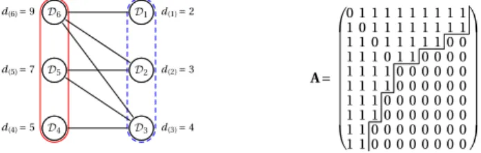
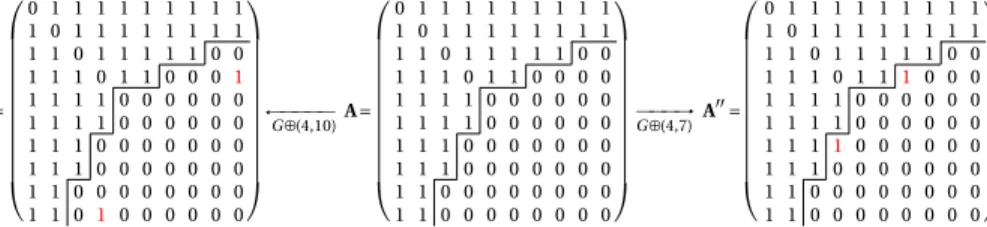
Figure1. Representation of a connected nested split graph (left) and the associated adjacency matrix (right) withn=10agents and k=6distinct positive degrees. A line betweenDi and Djindicates that every node inDi is linked to every node inDj. The solid frame indicates the
dominating set, and the nodes in the independent sets are included in the dashed frame. Next to the setDi, the degree of the nodes in the set is indicated. The neighborhoods are nested such
that the degrees are given byd(i+1)=d(i)+ |Dk−i+1|fori= k/2andd(i+1)=d(i)+ |Dk−i+1| −1 fori= k/2. In the corresponding adjacency matrixA(on the right), the 0 entries are separated from the 1 entries by a step function.
Definition4 (Mahadev and Peled 1995). Consider a nested split graphG=(NE)and letD=(D0D1 Dk)be its degree partition. Then the nodesN can be partitioned in independent setsDi,i=1 k/2, and a dominating setki=k/2+1Diin the graph G=(N \D0E). Moreover, the neighborhoods of the nodes are nested. In particular, for each nodev∈Di,i=1 k,
Nv= ⎧ ⎪ ⎪ ⎪ ⎪ ⎪ ⎪ ⎨ ⎪ ⎪ ⎪ ⎪ ⎪ ⎪ ⎩
i j=1
Dk+1−j ifi=1 k
2 i
j=1
Dk+1−j
{v} ifi=
k
2
+1 k.
Figure 1(left) illustrates the degree partition D=(D0D1 D6)and the nested neighborhood structure of a nested split graph. A line betweenDiandDjindicates that every node inDiis linked to every node inDj for anyi j=1 6. The nodes in the dominating set included in the solid frame induce a clique while the nodes in the inde-pendent sets that are included in the dashed frame induce an empty subgraph. In the following discussion, we will call the setsDi,i= k/2 +1 k,dominating subsets, since the setDiinduces a dominating set in the graph obtained by removing the nodes in the setkj=−0iDjfromG.
A nested split graph has an associated adjacency matrix that is called astepwise ma-trixand it is defined as follows.
Definition5 (Brualdi and Hoffman 1985). A stepwise matrixAis a symmetric, binary (n×n)matrix with elementsaij satisfying the following condition: ifi < jandaij=1, thenahk=1wheneverh < k≤jandh≤i.
Figure 1(right) shows the stepwise adjacency matrixAcorresponding to the nested split graph shown on the left hand side. If we let the nodes be indexed by the order of the
rows in the adjacency matrixA, then it is easily seen that, for example,D6= {12∈N:
d1=d2=d(6)=9}andD1= {910∈N:d9=d10=d(1)=2}.
If a nested split graph is connected, we call it a connected nested split graph. The representation and the adjacency matrix depicted inFigure 1actually show a connected nested split graph. From the stepwise property of the adjacency matrix, it follows that a connected nested split graph contains at least one spanning star, that is, there is at least one agent that is connected to all other agents. InAppendix C, we also derive the clustering coefficient, the neighbor connectivity, and the characteristic path length of a nested split graph. In particular, we show that connected nested split graphs have small characteristic path length, which is at most2. We also analyze different measures of centrality (seeWasserman and Faust 1994, Chapter 5.2) in a nested split graph. One important result is that degree, closeness, and Bonacich centrality induce the same or-dering of nodes in a nested split graph. If the oror-dering is not strict, then this holds also for betweenness centrality (seeAppendix C.2.5).
In the next proposition, we identify the relationship between the Bonacich centrality of an agent and her degree in a nested split graph. Denote byG⊕(i j)the networkG for which a link betweeniandjhas been added, and denote byG(i j)the networkG for which the link betweeniandjhas been deleted.
Proposition1. Consider a pair of agentsi j∈N of a nested split graphG=(NE). (i) If and only if agentihas a higher degree than agentj, thenihas a higher Bonacich
centrality thanj, i.e.,di> dj⇔bi(G λ) > bj(G λ).
(ii) Assume that neither the links(i k)nor(i j)are inG,(i j) /∈Eand(i k) /∈E. Fur-ther assume that agentkhas a higher degree than agentj,dk> dj. Then adding
the link(i k)toGincreases the Bonacich centrality of agentimore than adding the link(i j)toG, i.e.,dk> dj⇔bi(G⊕(i k) λ) > bi(G⊕(i j) λ).
(iii) Consider two agentsj k∈Niand assume that agentkhas a higher degree than
agent j, dk> dj. Then removing the link (i k) fromGdecreases the Bonacich
centrality of agent i more than removing the link(i j) fromG, i.e., dk > dj ⇔ bi(G(i k) λ) < bi(G(i j) λ).
From part (ii) ofProposition 1, we find that when agentihas to decide to create a link to either agentkorj, withdk> dj, in the link formation process(G(t))t∈R+, then iwill always connect to agentkbecause this link givesia higher Bonacich centrality than the other link to agentj. A similar argument holds for the removal of a link in part (iii). We can make use of this property to show that the networks emerging from the link formation process defined in the previous section actually are nested split graphs. This result is stated in the next proposition.
Proposition2. Consider the unperturbed dynamics of the network formation process
(G(t))t∈R+introduced inDefinition 2. Assume that att=0, we start with the empty net-workG(0)= ¯Kn. Then, at any timet≥0, the networkG(t)is a nested split graph almost
surely and the set∈, consisting of all possible unlabeled nested split graphs onnnodes with|| =2n−1, has measureP()=1.
This result is due to the fact that agents, when they have the possibility of creating a new link, always connect to the agent who has the highest Bonacich centrality (and byProposition 1the highest degree). This creates a nested neighborhood structure that can always be represented by a stepwise adjacency matrix after a possible relabeling of the agents.20The same applies for link decay.
Let us give some more intuition of this crucial result. Agents want to link to oth-ers who are more central since this leads to higher actions (as actions are proportional to centrality) and higher actions raise payoffs more. Similarly, links decay to those with lower centrality as these agents have lower actions and hence lower payoff effects. Notice, moreover, that once a link decays to an agent, she becomes less central and this makes it more likely that another link decays. Thus link gains and losses are self-reinforcing. This intuition suggests that if α, the probability of adding links, is large, then the process should approximate the complete network, while if it is small, then the process should approximate the star network. The key insight of our model is that for intermediate values ofα, the network is a nested split graph.
Observe that it is assumed that there is no cost of forming links. If links represent a social tie, then there typically is a cost to maintaining a link since agents must spend time with the person they are linked to. Because of the assumption of the absence of any linking cost, each agent wants to connect to every other agent, which leads to the formation of nested split graphs. InAppendix E, we extend the model to see what would happen to our results if links were costly to maintain and only the links that increase the payoff of an agent were formed. We show that as long as the cost is not too high, marginal payoffs are positive and the networks always converge to nested split graphs so that all our results hold.
Due to the nested neighborhood structure of nested split graphs, any pair of agents in (the connected component of ) a nested split graph is at most two links separated from each other. FromProposition 1it then follows that in a nested split graphG(t), the best response of an agentiis the agents with the highest degrees ini’s second-order neighborhoodNi(2).21 Moreover, ifG(t)is a nested split graph, theni∈Bj(G(t))if and only ifj∈Bi(G(t)). Hence, we could require in addition that links are only formed under mutual consent.
From the fact thatG(t)is a nested split graph with an associated stepwise adjacency matrix, it further follows that at any timetin the network evolution,G(t)consists of a single connected component and possibly isolated nodes.
Corollary 1. Consider the unperturbed dynamics of the network formation process
(G(t))t∈R+introduced inDefinition 2. Assume that att=0, we start with the empty net-workG(0)= ¯Kn. Then, at any timet≥0, the networkG(t)has at most one nonsingleton
component almost surely.
20Further, we will show inProposition 3that asζconverges to zero,(G(t))
t∈R+ induces a finite state
Markov chain where the recurrent statesˆ consist of nested split graphs.
21LetN
i= {k∈N:(i k)∈E(t)}be the set of neighbors of agenti∈Nand letNi(2)=j∈NiNj\(Ni∪ {i}) denote the second-order neighbors of agentiin the current networkG(t). Note that the connectivity rela-tion is symmetric such thatjis a second-order neighbor ofiifiis a second-order neighbor ofj, i.e.,i∈N(2) j
Nested split graphs are not only prominent in the literature on spectral graph the-ory, but they have also appeared in the recent literature on economic networks. Nested split graphs are called interlinked stars inGoyal and Joshi (2003).22Subsequently,Goyal et al. (2006)identified interlinked stars in the network of scientific collaborations among economists. It is important to note that nested split graphs are characterized by a dis-tinctive core–periphery structure (see theIntroduction(Section 1) andSection 6).
Finally, note that the network formation process(G(t))t∈R+ introduced in
Defini-tion 2is independent of initial conditionsG(0).23 This means that even when we start from an initial networkG(0)that is not a nested split graph, then after some finite time the Markov chain will reach a nested split graph. This is because there exists a positive probability that all links in the current graph are removed. The resulting graph is then empty. This graph is a special case of a nested split graph. Due toProposition 2forζ=0, from then on all consecutive networks visited by the chain are nested split graphs and the class of nested split graphs will never be left by the chain, that is, it forms an absorb-ing set. Moreover, since the chain stays forever in the class of nested split graphs and it takes only a finite number of transitions to reach this class from any other graph, all other graphs form a transient set.
4. Stochastically stable networks: Characterization
In this section, we show that the network formation process(G(t))t∈R+ ofDefinition 2
induces an ergodic Markov chain with a unique invariant distribution. We then proceed by analyzing the stochastically stables states inˆ (in the limit ofζ→0) of this process as the numbernof agents becomes large.
Proposition 3. The network formation process(G(t))t∈R+ introduced inDefinition 2 induces an ergodic Markov chain on the finite state spacewith a unique stationary dis-tributionμζsuch thatμζ(G)=limt→∞P(G(t)=G|G(0)=G)for anyG G∈.
More-over, the stochastically stable statesˆ are given by the set of nested split graphssuch thatμ()=1.
In the following discussion, we will assume for simplicity that αi=1−βi=α for alli∈N inDefinition 2, expressing the relative weights of link creation versus link de-cay.24 In this case, the symmetry of the network formation process with respect to the link arrival rateα and the link decay parameter1−α allows us to state the following proposition.
Proposition4. Consider the unperturbed dynamics of the Markov chain(G(t))t∈R+ in
Definition 2withα≡αi=1−βifor alli∈N. LetG(t)be a sample path generated with 22Nested split graphs are interlinked stars, but an interlinked star is not necessarily a nested split graph.
Nested split graphs have a nested neighborhood structure for all degrees, while in an interlinked star, this holds only for the nodes with the lowest and highest degrees.
23SeeProposition 3inSection 4and its proof inAppendix A.
24Note that taking into account the possibility of an agent remaining quiescent only modifies the time
scale of the process discussed, thus yielding identical results to the model proposed. This implies that, without any loss of generality, it is possible to assumeαi+βi=1for alli∈N. For simplicity, we also
the homogeneous link arrival rateαand letG(t)be a sample path with arrival rate1−α. Let μbe the stationary distribution of G(t)and letμ be the stationary distribution of
G(t). Then for each networkGin the support ofμ, the complementG¯ ofGhas the same probability inμ, i.e.,μ(G)¯ =μ(G).
Proposition 4 allows us to derive the stationary distribution μ for any value of 1
2< α <1if we know the corresponding distribution for1−α. This follows from the fact that the complementG¯ of a nested split graphGis a nested split graph as well (Mahadev and Peled 1995). In particular, the networksG¯ are nested split graphs in which the num-ber of nodes in the dominating subsets corresponds to the numnum-ber of nodes in the in-dependent sets inGand, conversely, the number of nodes in the independent sets inG¯ corresponds to the number of nodes in the dominating subsets inG.
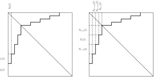
With this symmetry in mind, we restrict our analysis in the following discussion to the case of 0< α≤ 12. Let {N(t)}t∈R+ be the degree distribution with thedth
ele-ment Nd(t), giving the number of nodes with degree d inG(t), in the tth sequence
N(t)≡ {Nd(t)}dn=−10. Further, let Pt(d)≡Nd(t)/n denote the proportion of nodes with degreed (P(t)≡N(t)/n) and let P(d)≡limt→∞Pt(d) be its asymptotic value. In the following proposition, we determine the asymptotic degree distribution of the nodes in the independent sets fornlarge enough.25
Proposition5. Consider the unperturbed dynamics of the Markov chain(G(t))t∈R+ in
Definition 2withα≡αi=1−βifor alli∈N and let0< α≤12. LetPt(d)denote the
pro-portion of nodes with degreedinG(t). Then the asymptotic expected proportion of nodes in the independent sets with degreesd=01 d∗in the stochastically stable networks
G∈ ˆfor largenis given by lim
t→∞E(Pt(d))=
1−2α
1−α α
1−α d
(3)
where26
d∗(n α)=ln
(1−2α)n 2(1−α)
ln1−αα (4)
andPt(d)→Et(Pt(d))almost surely asn→ ∞.
The proof of the proposition follows from a series of intermediate steps, where we can take advantage of the intuitively simple stepwise structure of the adjacency matrix associated with a nested split graph (seeFigure 1). First we use the fact that we can ap-proximate the continuous time Markov chain with a sampled time Markov chain whose stationary distributions are the same (seeLemma 1inAppendix A). We then proceed 25AsProposition 5speaks of the asymptotic degree distribution in the limit of largen, this is to be
under-stood as lettingn→ ∞after considering the limit oft→ ∞.
26Note thatd∗(n α)from (4) might, in general, not be an integer. In this case, we take the closest integer value to (4), that is, we take[d∗(n α)] = d∗(n α)+1
2. The error we make in this approximation is negligible for largen.
by induction to show that (3) holds for all degrees smaller than an upper boundd∗in the support of the stationary distribution μ of the sampled time Markov chain. The induction basis is concerned with the number of isolated nodes (separately derived in Lemma 3inAppendix A) and the number of nodes with degree1. The induction step assumes that (3) holds ford−1anddto show that it then must also hold ford+1. To draw this conclusion, we compute the fixed point of the expected change in the number of nodes with degreedin an incremental time step using the fact that the underlying network is a nested split graph. This is possible because of the particular structure in-herent in the adjacency matrix of a nested split graph and our payoff maximizing link formation protocol, which allows us to consider only a few cases for the formation or re-moval of a link to compute that change. Finally, by requiring that the degree distribution is a proper probability measure with mass1, we can derived∗in (4). The details of the proof can be found inAppendix A.
The structure of nested split graphs implies that if there exist nodes for all degrees between0andd∗(in the independent sets), then the dominating subsets with degrees larger thand∗contain only a single node. Further, usingProposition 4, we know that for α >12, the expected number of nodes in the dominating subsets is given by the expected number of nodes in the independent sets in (3) for1−α, while each of the independent sets contains a single node. This determines the asymptotic degree distribution for the independent or dominating subsets, respectively, for all values ofαin the limit of largen.
From (4), we can directly derive the following corollary.
Corollary 2. Consider the unperturbed dynamics of the Markov chain(G(t))t∈R+ in
Definition 2withαi=1−βi=αfor alli∈N. Then there exists a phase transition in the
asymptotic average number of independent sets,d∗(n α), forG∈ ˆasnbecomes large such that
lim
n→∞
d∗(n α) n =
⎧ ⎪ ⎨ ⎪ ⎩
0 ifα <12 1
2 ifα= 1 2 1 ifα >12.
Corollary 2implies that asngrows without bound, the networks in the stationary distributionμ are either sparse or dense, depending on the value of the link creation probabilityα. Moreover, from the functional form ofd(n α)in (4), we find that there exists a sharp transition from sparse to dense networks asαcrosses12and the transition becomes sharper the larger isn.
Observe that because a nested split graph is uniquely defined by its degree distribu-tion,27Proposition 5delivers us a complete description of a typical network generated by our model in the limit of largetandn. We call this network thestationary network. We can compute the degree distribution and the corresponding adjacency matrix of the stationary network for different values ofα.28 The latter is shown inFigure 2. From the 27The degree distribution uniquely determines the corresponding nested split graph up to a permutation
of the indices of nodes.
28Noninteger values for the partition sizes can be approximated with the closest integer while preserving
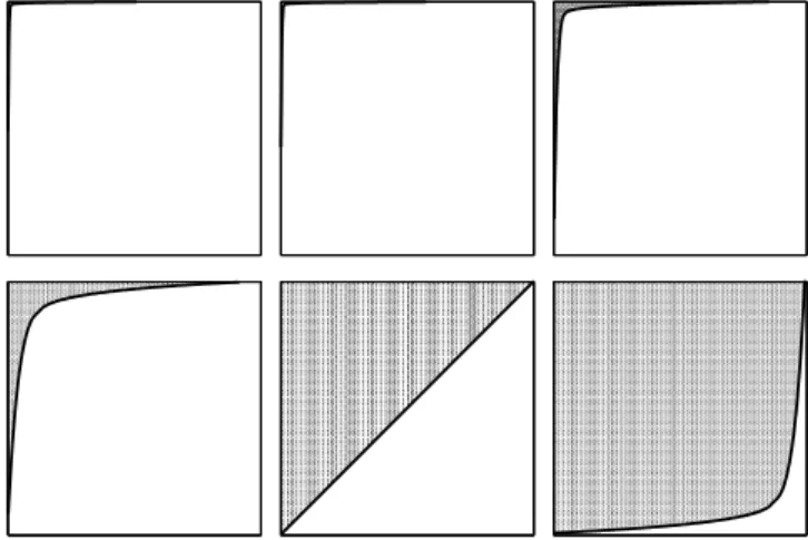
Figure 2. Representation of the adjacency matrices of stationary networks with n=1,000
agents for different values of parameter α: α=02(top-left plot), α=04(top-center plot),
α=048(top-right plot),α=0495(bottom-left plot),α=05(bottom-center plot), andα=052
(bottom-right plot). The solid line illustrates the step function separating the0from the1 en-tries in the matrix. The top-left matrix forα=04corresponds to a starlike network while the bottom-right matrix forα=052corresponds to an almost complete network. Thus, there ex-ists a sharp transition from sparse to densely connected stationary networks around α=05. Networks of smaller size for the same values ofαcan be seen inFigure 3.
structure of these matrices, we observe the transition from sparse networks containing a hub and many agents with small degree to a quite homogeneous network with many agents having similar high degrees. Moreover, this transition is sharp aroundα=12. In Figure 3, we show particular networks arising from the network formation process for the same values ofα. Again, we can identify the sharp transition from hub-like networks to homogeneous, almost complete networks.
Figure 4(left) displays the numberm¯ of linksmrelative to the total number of pos-sible linksn(n−1)/2, i.e.,m¯ =2m/(n(n−1)), and the number of distinct degreeskas a function ofα. We see that there exists a sharp transition from sparse to dense net-works aroundα=12, whilekreaches a maximum atα= 12. This follows from the fact thatk=2d∗withd∗given in (4) is monotonic increasing inαforα < 12and monotonic decreasing inαforα >12.
Note thatProposition 5makes a statement in the limit ofn→ ∞. In the following section (see in particular Figures4–8), we compare various networks statistics computed from the analytical solution inProposition 5with the results obtained from numerical simulations for finite values ofn. These figures illustrate that for relatively small values of nthere is almost no deviation from the theoretical prediction ofProposition 5, providing evidence that our limit results also make reasonably good predictions in the case of a finite numbernof agents.29
29This also weakens the eigenvalue condition imposed on the spillover parameterλintroduced in Sec-tion 3.1. See alsofootnote 10.
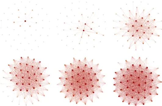
Figure 3. Sample networks withn=50agents for different values of parameterα: α=02
(top-left plot),α=04(top-center plot),α=048(top-right plot),α=0495(bottom-left plot),
α=05(bottom-center plot), andα=052(bottom-right plot). The shade and size of the nodes indicate their eigenvector centrality. The networks for small values ofαare characterized by the presence of a hub and a growing cluster attached to the hub. With increasing values ofα, the density of the network increases until the network becomes almost complete.
5. Stochastically stable networks: Statistics
In the following sections, we analyze some of the topological properties of the stochas-tically stable networks in our model that are in the support of the stationary distribu-tionμ. We simply refer to these networks as stationary networks. With the asymptotic expected degree distribution derived in Proposition 5, we can calculate the expected clustering coefficient, the clustering-degree correlation, the neighbor connectivity, the assortativity, and the characteristic path length by using the expressions derived for these quantities inAppendix C, where we show that these statistics are all functions of the degree distribution.30
Note that since the stationary distributionμis unique, we can recover the expected value of any statistic by averaging over a large enough sample of empirical networks generated by numerical simulations. We then superimpose the analytical predictions of the statistic derived fromProposition 5with the sample averages so as to compare the validity of our theoretical results, also for small network sizesn. As we will show, there is a good agreement of the theory with the empirical results for alln.
30Any network statistic f:→R we consider can be expressed as a function of the
(empir-ical) degree distribution Pt:→ [01]n. Hence, we can compute the expectation as Et(f )=
k∈(0n)nf (k/n)Pt(Pt=k/n). InProposition 5, we show that the degree distribution converges to its
ex-pected value with probability1. Therefore, we have thatEt(f )=k∈(0n)nf (k/n)1Et(Pt)(k/n)=f (Et(Pt))
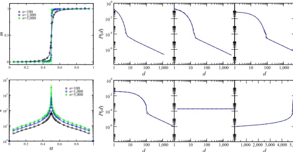
Figure4. (Left) In the top panel we show the numberm¯ of linksmrelative to the total number of possible linksn(n−1)/2of the stationary network. The number of distinct degreesk=2d∗, withd∗from (4), found in the stationary network for different values ofαare shown in the bot-tom panel. The figures display both the results obtained by recourse of numerical simulations (symbols) and by respecting theoretical predictions (lines) of the model. (Right) Degree distribu-tionP(d)for different values of parameterαand a network sizen=10,000:α=02(top-left plot),
α=04(top-center plot),α=048(top-right plot),α=049(bottom-left plot),α=05(bottom– center plot), andα=052(bottom-right plot). The solid line corresponds to the average of sim-ulations, while the dashed line indicates the theoretical degree distribution fromProposition 5. The degrees have been binned to smooth the degree distribution.
We would like now to investigate the properties of our networks and see how they match real-world networks.
Degree distribution
FromProposition 5, we find that the degree distribution follows an exponential decay with a power-law tail.31 The power-law tail has an exponent of−1.32 Figure 4displays the relative degree in the network (left panel) and the degree distribution (right panel).
31For0< α≤1
2andnlarge enough, the asymptotic expected degree distribution for the degreesdsmaller than or equal tod∗is given by an exponential functionP(d)=((1−2α)/(1−α))exp(−ln((1−α)/α)d). On the other hand, if we assume (i) that the degree of a node in a dominating subset is symmetrically distributed around its expected value, (ii) we compute the integral over the probability density function by a rectangle approximation, and (iii) we further assume that the degree distribution obtained in this way has the same functional form for all degreesdlarger thand∗, then one can show that for0< α≤1
2andn large enough, the asymptotic expected degree distributionP(d)is given byP(d)=(α/((1−2α)n))d−1. The power-law tail of the degree distribution can be confirmed by the empirical distribution from a logarithmic binning of numerical simulations, as can be seen inFigure 4(right).
32We can extend our model to obtain a degree distribution with an arbitrary power-law tail by making the
Figure 5. The left panel shows the clustering coefficientC and the right panel the cluster-ing-degree correlation of stationary networks. The symbols correspond to the results obtained by recourse of numerical simulations. The solid lines correspond to the analytical results. We show that the clustering-degree correlation is negative for different values ofαand a network size ofn=1,000. The different plots show different values ofα: α=02(top-left plot),α=04
(top-center plot),α=048(top-right plot),α=049(bottom-left plot),α=05(bottom-center plot), andα=052(bottom-right plot).
Figure6. In the left panel, we show the assortativityγ of stationary networks. In the right panel, we show the average nearest neighbor connectivitydnnforα=02(top-left plot),α=04
(top-center plot),α=048(top-right plot),α=049(bottom-left plot),α=05(bottom-center plot), andα=052(bottom-right plot). The symbols correspond to the results obtained by re-course of numerical simulations. The solid lines correspond to the analytical results.
Clustering
The clustering coefficient is shown inFigure 5(left). We find that for practically all values ofα, the clustering in the stationary networks is high. This finding is in agreement with
structure of the network she is embedded in. This extension is further discussed inKönig and Tessone (2011).
Figure7. (Left panel) The characteristic path lengthof stationary networks and (right panel) the results for the network efficiency, obtained by recourse of numerical simulations (symbols) and respecting theoretical predictions (lines) of the model.
Figure8. (From left to right) Degree, closeness, betweenness, and eigenvector centralization in the stationary networks for different values ofα. For all centralization measures, we obtain a sharp transition between strongly centralized networks for lower values ofαand decentralized networks for higher values ofα. Note that we have only considered the connected component for the computation of the different centralization measures.
the vast literature on social networks that has reported high clustering to be a distinctive feature of social networks. Moreover,Goyal et al. (2006)have shown that there exists a negative correlation between the clustering coefficient of an agent and her degree. We find this property in the stationary networks as well, as it is shown inFigure 5(right).
Assortativity and nearest neighbor connectivity
We now turn to the study of correlations between the degrees of the agents and their neighbors. This property is usually measured by the network assortativityγ(Newman 2002)33and nearest neighbor connectivitydnn(d)(Pastor-Satorras et al. 2001). Dissor-tative networks are characterized by negative degree correlations between a node and 33The assortativity coefficientγ∈ [−11]is essentially the Pearson correlation coefficient of degree
be-tween nodes that are connected. Positive values ofγindicate that nodes with similar degrees tend to be connected (anddnn(d)is an increasing function of the degreed), while negative values indicate that nodes
with different degrees tend to be connected (anddnn(d)is a decreasing function of the degreed). See Newman (2002)for further details.
its neighbors, and assortative networks show positive degree correlations. In dissorta-tive networks, γis negative and dnn(d) is monotonic decreasing, while in assortative networksγis positive anddnn(d)is monotonic increasing. In our model, we observe dissortative networks.34
Assortativity and average nearest neighbor connectivity for different values of the link creation probabilityαare shown inFigure 6. Clearly, stationary networks are dissor-tative, while the degree of dissortativity decreases with increasingα. The dissortativity of stationary networks simply reflects the fact that stationary networks are strongly cen-tralized for values ofαbelow12.
Characteristic path length
Figure 7shows the characteristic path lengthand the network efficiency(defined in Appendix C.1.4). From these figures, one can see that the characteristic path length never exceeds a distance of2. Together with the high clustering shown in this section, the stationary networks can be seen as “small worlds” (Watts and Strogatz 1998). Sta-tionary networks are efficient for values ofα larger than 12, in terms of short average distance between agents, while for values ofαsmaller than12they are not. However, this short average distance is attained at the expense of a large number of links.
Centralization of stochastically stable networks
In the following section, we analyze the degree of centralization in stationary networks. For our analysis, we use the centralization index introduced byFreeman (1979). The centralizationC:→ [01]of a networkG=(NE)∈is given by
C≡
u∈G(C(u∗)−C(u))
maxGv∈G(C(v∗)−C(v))
where u∗ and v∗ are the agents with the highest values of centrality in the current network and the maximum in the denominator is computed over all networks G= (NE)∈with the same number of agents.
FromFigure 8(right), showing degree, closeness, betweenness, and eigenvector cen-tralization, we clearly see that there exists a phase transition atα= 12 from highly cen-tralized to highly decencen-tralized networks. This means that for low arrival rates of linking opportunitiesα(and a strong link decay), the stationary network is strongly polarized, composed mainly of a star (or an interlinked star as inGoyal and Joshi 2003), while for high arrival rates of linking opportunities (and a weak link decay), stationary networks are largely homogeneous. We can also see that the transition between these states is sharp. It is interesting to note that the same pattern emerges for all centrality measures considered, irrespective of whether the measures take into account only the local neigh-borhood of an agent, such as in the case of degree centrality, or the entire network struc-ture, as for the other centrality measures.
34InKönig et al. (2010), we show that by introducing capacity constraints in the number of links an agent
Figure9. The Austrian banking network, the global network of banks obtained from the Bank of International Settlements (BIS) locational statistics, the gross domestic product (GDP) trade network, and the arms trade network (from left to right). The shade and size of the nodes indicate their eigenvector centrality. The GDP trade network is much more dense than the network of banks and the network of arms trade. All four networks show a core of densely connected nodes.
6. Empirical implications 6.1 Data
In this section, we would like to provide real-world evidence for our model and estimate the model’s parameters for four different empirical data sets, all of which are charac-terized by a strongly nested network architecture. We essentially consider two types of networks: bank and trade networks.35 In the following discussion, we describe in detail the different data sets that we use.
The first network we analyze is a network of Austrian banks in the year 2008 (see Boss et al. 2004). Links in the network represent exposures between Austrian-domiciled banks on a nonconsolidated basis (i.e., no exposures to foreign subsidiaries are in-cluded). We obtain a sample ofn=770banks withm=2,454links between them and an average degree ofd¯=2054. The degree variance isσd2=1,27322. The largest con-nected component comprises768banks, which is997%of the total of banks, and it is illustrated inFigure 9.
Second, we consider the global banking network in the year 2011 obtained from the Bank of International Settlements (BIS) locational statistics on exchange-rate-adjusted changes in cross-border bank claims (seeMinoiu and Reyes 2011). BIS locational statis-tics are compiled on the basis of residence of BIS reporting banks and cover the cross-border positions of all banks domiciled in the reporting area, including positions with respect to foreign affiliates, loans, deposits, debt securities, and other assets provided by banks. We obtain a network withn=239nodes andm=2,454links between them. An illustration can be seen inFigure 9. The average degree of the network isd¯=2054and we observe a high degree variance ofσ2
d=1,27322.
The third empirical network we consider is the network of trade relationships be-tween countries in the year 2000. The trade network is defined as the network of import– export relationships between countries in a given year in millions of current-year U.S. 35InAppendix D, we discuss an application of our model to networks of banks (seeAppendix D.1), where
links are loans between banks, and in terms of trade networks (seeAppendix D.2), where links between countries represent trade relationships (in imports or exports).