VOLUME 16 ISSUE 3 (2018) Page 221 – 232
GIS-BASED REGRESSION ANALYSIS OF THE RELATIONSHIP BETWEEN ECOLOGICAL FOOTPRINT AND ECONOMIC
DEVELOPMENT OF SELECTED COUNTRIES
M.Rafee Majid1, Musarrat Zaman2 & Norhazliza Halim3
Faculty of Built Environment UNIVERSITI TEKNOLOGI MALAYSIA
Abstract
Ecological footprint is an innovative concept to present the consumption of natural resources and generation of waste in terms of the Earth biological carrying capacity in a standardized format. The Earth overall sustainability can also be measured with the idea of ecological footprint and bio-capacity. The aim of this paper is to analyse the interactive spatial relationship between economic development and ecological footprints of selected nations. The GIS-based spatial regression tool Ordinary Least Square (OLS) and Geographically Weighted Regression (GWR) are used for fulfilling the purpose. Individual components of ecological footprints - cropland, grazing land, fishing ground, forest land, built-up land and carbon footprints - are also analysed against the per capita GDP of the nations in order to understand the interrelationship between them. The analysis has found a significant relationship between ecological footprint and economic development and the OLS model can explain approximately 64% of the variation in the dependent variable with the explanatory variables. The study has also found that nation’s economic development contributes much in increasing the carbon footprint. The resulted outcome is significant enough to warrant a study on the spatial dimension of environment and economy in order to analyse the individual nation’s economic growth and its relationship with environmental degradation, which can ultimately influence the global environmental sustainability.
Keywords: ecological footprint, economic development, sustainability,
INTRODUCTION
There is always an integrated relationship between economic growth and environmental impact on the development of human civilization. Natural ecosystem is one of the major components of the environment that has an inevitable connection with the economic activities (Wang, Kang, Wu & Xiao, 2013) and the needs of human are supposed be met through balancing the ecological components without compromising the health of ecosystems (Callicott & Mumford, 1997). However, overconsumption of natural assets can turn into the degradation of ecological system services in general and leads towards the depletion that can hardly be restored (MEA, 2005). In this situation, the sustainability of the environment cannot be ensured. In order to seek balance between these two factors, a considerable interest in analysing this interrelationship has been geared up among researchers over the past decadesand the idea of ecological footprint was developed.
Ecological footprint is an important concept that estimates the Earth biological carrying capacity required to support the resource use of human and their produced waste in a standardized format (Venetoulis & Talberth, 2008). According to Wackernagel et al. (2005), ecological footprint measures how much of the annual regenerative capacity of the biosphere is required to renew the resource input of a defined population in a given year. The total productive land area is calculated on Global Hectare (GHA) unit that supplies the natural resources and processes the wastes of a particular entity. Ecological footprint is most commonly used to estimate a nation’s consumption in National Footprint Accounts (NFAs), consisting the aggregate result of six individual sectors made up of cropland footprint, grazing footprint, forest land, carbon footprint, fish footprint and total built up land (Lin et al., 2016).
measure the interrelationship of cropland, grazing land, forest land, carbon, fish ground and total built up land footprints with the per capita GDP of the selected countries.
DATA AND METHODS
This study is based on the fundamentals of linear regression analysis. The specific data regarding ecological footprints and other economic and socio-economic factors of the countries are collected from online sources. National Footprint Accounts (NFAs) Data Package of the global nations calculated by Global
Footprint Network (GFN) organization is downloaded from
www.footprintnetwork.org. In the year 2012, the NFAs calculated the Footprints of 232 countries, territories, and regions from 1961 to the present. This Data Package contains ecological footprint and bio-capacity data including cropland footprint, grazing footprint, carbon footprint, fish footprint, total built up land and total EF and bio-capacity data for year 2012; HDI and total population of the countries; per capita GDP; level of income group of the countries within the year 2012. Again for the indicator of income inequalities, the latest Gini Index of the respective countries is downloaded from World Bank’s website (World Bank, 2017). The world vector map consisting the shape files of each country is downloaded from Thematic Mapping Website (thematicmapping, n.d.).
The GIS-based multiple regression analysis is the key analysis of this research. The data analysis of this study is based on Ordinary Least Square Regression (OLSR) as well as Geographically Weighted Regression (GWR) for fulfilling the first objective. Statistical and spatial analysis are done on both the software of ArcGIS and MS Excel. For that Ordinary Least Square Analysis and Geographically Weighted Regression Analysis tools are used. Only 203 out of 232 countries are analysed for OLSR and GWR, due to missing data in the other 29 countries. For the multiple regression analysis on MS Excel, only 161 countries are considered.
Ordinary Least Squares (OLS) linear regression is a global regression model that can generate predictions and model the relationship of a dependent variable in terms of a set of explanatory variables. It determines the heteroscedasticity or non-stationarity of the global data and confirms the applicability of GWR for further steps. The basic equation is as follows:
Y= β0+β1X1+ β2X2+……… βnXn+ε (1)
respective coefficient is positive if the relationship is positive whereas negative relationships is expressed with negative signs of the coefficients.
Global OLS calculates various statistics and makes the validity of transferring in GWR analysis through the model performance assessments, assessment of each explanatory variable in the model (coefficient, probability or robust probability, and variance inflation factor (VIF), model significance assessment, stationarity assessment, model biasness assessment and residual spatial autocorrelation assessment). If the model proven to be non-stationary or spatial heterogeneity, then GWR can be applied for the next analysis. The spatial heterogeneity is then analysed using the sophisticated tool of ArcGIS, which is known as Geographically Weighted Regression (GWR). It is local regression model for analysing the spatial heterogeneity. If the modelled structure of the process varies across the study area, the spatial heterogeneity occurs.
RESULTS AND DISCUSSION
Relationship between Per Capita GDP, HDI, Income Inequality and Total Population with the Ecological Footprint
Ordinary Least Square (OLS) tool was used for performing global regression analysis in ArcGIS. The shapefile of the global map including the necessary attribute table was given as input feature class. The Unique ID Field was given as UN, which is a unique integer number of the attribute table. Countries’ total ecological footprint was the dependent variable whereas HDI, Per capita GDP, Population size and Gini Index were explanatory variables.
The OLSR was operated on the variables of total 203 observations and produced detail analysis report on the observations and operation. According to the values of coefficient of the explanatory variables, intercept and standard residuals, an equation of the model was formed as follows;
EF=1.295+2.702HDI+0.000071PER_CAPITA_GDP-.000228POPULATION-0.024569GINI_INDEX (2)
It provided various information and interpretation techniques for the generated statistics. Firstly, it shows the Akaike Information Criterion (AIC) value. The AIC (Akaike Information Criterion) is an estimator of the relative quality of statistical models regularly used as a means for model selection. It estimates the quality of each model, relative to each of the other models. Lower AIC value is preferred over higher one. For this model, the AIC was quite small (718.5).
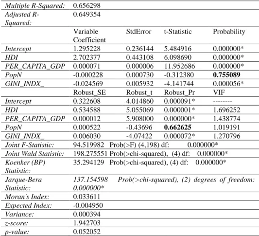
1 shows that, the multiple R-squared value was 0.656 and adjusted R-Squared value was 0.649. These indicate that the model explains approximately 65% of the variation in the dependent variable. This value will be increased if more explanatory variables were added. Again, the coefficient for each explanatory variable reflects both the strength and type of relationship it has with the dependent variable. Table 1 shows that among the four explanatory variables, HDI and Per Capita GDP have positive correlation with the dependent variable. That means if either the HDI or per capita GDP of the countries risen, the ecological footprint of the countries would also increase. On the other hand country’s total population and Gini coefficient have slightly negative relationship with the ecological footprint (-0.000228 and -0.024569). That can be interpreted as, if the Gini coefficient values and number of population increased, the ecological footprint will decrease.
Table 1: Outcome statistics of OLSR analysis in ArcGIS
Multiple R-Squared: 0.656298
Adjusted R-Squared:
0.649354
Variable Coefficient
StdError t-Statistic Probability
Intercept 1.295228 0.236144 5.484916 0.000000*
HDI 2.702377 0.443108 6.098690 0.000000*
PER_CAPITA_GDP 0.000071 0.000006 11.952686 0.000000*
PopN -0.000228 0.000730 -0.312380 0.755089
GINI_INDX_ -0.024569 0.005932 -4.141744 0.000056*
Robust_SE Robust_t Robust_Pr VIF
Intercept 0.322608 4.014860 0.000091* ---
HDI 0.534588 5.055069 0.000001* 1.696252
PER_CAPITA_GDP 0.000012 5.908000 0.000000* 1.438774
PopN 0.000522 -0.43696 0.662625 1.019191
GINI_INDX_ 0.006030 -4.07422 0.000072* 1.270796
Joint F-Statistic: 94.519982 Prob(>F) (4,198) df: 0.000000*
Joint Wald Statistic: 198.275551 Prob(>chi-squared), (4) df: 0.000000*
Koenker(BP)
Statistic:
35.294129 Prob(>chi-squared), (4) df: 0.000000*
Jarque-Bera Statistic:
137.154598 Prob(>chi-squared), (2) degrees of freedom:
0.000000*
Moran's Index: 0.033611
Expected Index: -0.004950
Variance: 0.000394
z-score: 1.942703
T-test was used to assess whether or not an explanatory variable was statistically significant. In this model, for three explanatory variables (HDI, Per Capita GDP and Gini index), the p value of the t-statistics was less than 0.05, which indicates that these variables were statistically significant for explaining ecological footprint. On the other hand, total population of the country did not have significant statistical relationship with the total ecological footprint; the possible reason has been discussed in the previous section.
In addition, the variance inflation factor (VIF) measures redundancy among explanatory variables. In this model, there was no such variable with the VIF value greater than 7.5. So, none of the variables needs to be excluded from the model.
Both the Joint F-Statistic and Joint Wald Statistic are measures of overall model statistical significance. The Joint F-Statistic is trustworthy only when the Koenker (BP) statistic is not statistically significant. If the Koenker (BP) statistic was significant, the Joint Wald Statistic should be consulted to determine overall model significance. Table 1shows that the probability values for all three of the F-statistics, Wald statistics and Koenker (BP) statistics were less than 0.05, which means the model is statistically significant and has a statistically significant heteroscedasticity or non-stationarity. As, regression models with statistically significant non-stationarity are especially good candidates for GWR analysis, from the OLS model, it can be preferred that GWR analysis will have a significant result using these three variables except country’s total population.
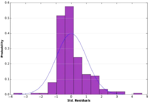
Figure 1: Histogram showing the normal distribution of standardized residuals
The outcome of OLS model indicates that the GWR analysis will have a significant result using the three variables HDI, per capita GDP and Gini index, except country’s total population. The following section discusses about the result outcome of GWR analysis and the interpretation of it.
Once the OLSR was done, GWR analysis was quick and easy to calculate. It is the local regression analysis which shows the spatial heterogeneity and non-stationarity. The geoprocessing tool is found in the same spatial statistics toolbox along with OLSR. In this study, GWR applied the AICc method using 30 neighbours to calibrate each local regression equation to yield optimal results by minimizing biasness and maximizing model fit. The AICc is the AIC estimator corrected for small sample sizes to address potential overfitting. The Adjusted R2
value was higher for GWR than it was for the OLS model (OLS was 65%; GWR was 67.77%). The higher AICc value of the GWR model indicates that the model is better run in OLSR than GWR. So, in this case GWR did not have much significance on the outcome.
Identifying the Interrelationship between the Components of Ecological Footprint and Economic Development of the Selected Countries
analysis was conducted on MS Excel with the spreadsheet format of the data of Global Footprint Network. Among the six types of footprint, only carbon footprint showed the significant correlation with per capita GDP. The other five types of footprint did not have noticeable R2 values. Therefore, the following
equation shows the Carbon Footprint regression with per capita GDP of the countries.
Carbon Footprint = 0.715+ 0.08001 PER_CAPITA GDP (3)
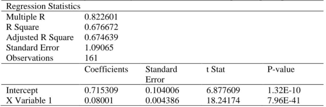
The carbon footprint of a nation measures the area of forest land required to sequester total carbon dioxide emissions of the nation. As per the regression result, countries have significant correlation of carbon footprint with their income level. From Table 2, it can be seen that for 161 observations, the Multiple R value was much higher than cropland footprint, which was 82%; R square and Adjusted R square values were around 67%, having standard error 1%. Again, the coefficient of correlation value was positive at 0.08, which means that the increase in per capita GDP contributes to greater amount of carbon emission and thus larger amount of forest land is required to sequester carbon dioxide.
Table 2: Output of regression analysis statistics of carbon footprint vs per capita GDP Regression Statistics
Multiple R R Square
Adjusted R Square Standard Error Observations
0.822601 0.676672 0.674639 1.09065 161
Coefficients Standard Error
t Stat P-value
Intercept X Variable 1
0.715309 0.08001
0.104006 0.004386
6.877609 18.24174
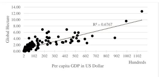
Figure 2: Scatterplot of the relationship between carbon footprint and per capita GDP of the nations
Figure 2 shows the relationship of carbon footprint and per capita GDP of the nations. It is clearly visible that countries with higher GDP have higher amount of carbon footprint. As, the higher income countries have greater demand for energy consumption due to the economic development, they contribute more to the carbon emission and global warming. The five other footprints like cropland footprint, grazing footprint, fishing ground footprint, forest land footprint did not have mentionable correlation with the per capita GDP. The overall result is exhibited in Figures 3 and 4, which present the relationship graphs of individual footprints and the per capita GDP.
Figure 3 shows the scatterplot graph of each footprint according to the level of GDP. The figure illustrates how the total ecological footprint of the countries increases with the increase in per capita GDP and the carbon footprints exceed all other footprints. Same scenario can be found on the average values of per capita GDP of the nations and their footprints as shown in Figure 4. From this figure it is easy to realize that lower income nations have lower percentage of total ecological footprints along with less percentage of individual components of it, whereas, the average total ecological footprint was greater in percentage for the higher income nations than the lower or lower middle and upper middle income countries.
R² = 0.6767
0.00 2.00 4.00 6.00 8.00 10.00 12.00 14.00
2 102 202 302 402 502 602 702 802 902 1002 1102
Glo
b
al
Hec
tar
e
Figure 4: Relationship between each footprint and per capita GDP according to the country income
CONCLUSION
Examining the relationship between ecological footprint and economic development indicators, it was found that ecological footprint of a country is directly proportional to its economic development. Per capita GDP of the nations was found to have significant correlation along with HDI. The other two variables, total population and income inequality, were found to have negative correlation with economic development, though their coefficients were very minor to be analysed. These mean that per capita GDP and HDI can better explain the change in ecological footprint compared to total population and income inequality. Countries with higher per capita GDP and HDI are more economically flourished and consume more resources. Their carbon emission is also greater than the lower income nations. As a result, carbon footprint represents a significant portion of the total ecological footprint than any other footprints. From the GWR, the OLSR model was modified and strengthened.
This study has a significant impact on understanding the interlink and variations among the ecological and economic factors to allow for further investigation of the way towards achieving sustainable environment. It provides the background information and conceptual framework for future studies related to economic development and environmental sustainability.
In conclusion, it can be inferred from the findings of this study that high economic development and wanton exploiting of natural resources have direct negative impacts on the ecological balance that also reduces the bio-capacity of nations. Thus, there must be a balance between the consumption of natural resources for economic growth and their conservation in order to achieve environmental sustainability.
0 1 2 3 4 5 6 7
High Income Upper Middle Income Lower Middle Income Low Income
global hectare
In
co
m
e
le
v
el
o
f t
h
e cou
n
trie
s
Cropland FTP Grazing Footprint Forest Product Footprint
REFERENCES
Anselin, L. (1998).GIS research infrastructure for spatial analysis of real estate markets.
Journal of Housing Research, 9(1), 113-133.
Callicott, J. B., & Mumford, K. (1997). Ecological sustainability as a conservation concept. Conservation Biology, 11(1), 32-40.
Lin, D., Hanscom, L., Martindill, J., Borucke, M., Cohen, L., Galli, A.,...& Wackernagel, M. (2016). Working Guidebook to the National Footprint Accounts: 2016
Edition. Oakland: Global Footprint Network.
Millennium Ecosystem Assessment [MEA]. (2005). Ecosystems and human well-being:
Synthesis. Washington, DC: Island Press.
thematicmapping (n.d.). World borders dataset. Retrieved February 10, 2017 from http:// thematicmapping.org/downloads/world_borders.php
Venetoulis, J., & Talberth, J. (2008). Refining the ecological footprint. Environment
Development and Sustainability, 10, 441-469.
Wackernagel, M., Monfreda, C., Moran, D., Wermer, P., Goldfinger, S., & Deumling, D. (2005). National footprint and biocapacity accounts 2005: The underlying calculation method. Land Use Policy, 21, 231-246.
Wang, Y., Kang, L., Wu, X., & Xiao, Y. (2013). Estimating the Environmental Kuznets curve for ecological footprint at the global level: A spatial econometric approach. Ecological Indicators, 34, 15-21.