LBS Research Online
K Ramdas, S A Atkinson and J W Williams
Robust scheduling practices in the U.S. airline industry: Costs, returns, and inefficiencies Article
This version is available in the LBS Research Online repository: http://lbsresearch.london.edu/
67/
Robust scheduling practices in the US airline industry
Ramdas, K, Atkinson, S A and Williams, J W (2016)
Robust scheduling practices in the U.S. airline industry: Costs, returns, and inefficiencies.
Management Science, 62 (11). pp. 3372-3391. ISSN 0025-1909
DOI:https://doi.org/10.1287/mnsc.2015.2302
INFORMS
http://pubsonline.informs.org/doi/10.1287/mnsc.201...
Robust Scheduling Practices in the U.S. Airline Industry: Costs,
Returns, and Inefficiencies.
Scott E. Atkinson∗ Kamalini Ramdas† Jonathan W. Williams‡
October 2014
Abstract
Airlines use robust scheduling to mitigate the impact of unforeseeable disruptions on prof-its. We examine how effectively three common practices – flexibility to swap aircraft, flexibility to reassign gates, and scheduled aircraft downtime – accomplish this goal. We first estimate a multiple-input multiple-outcome production frontier, which defines the attainable set of out-comes from given inputs. We then recover unobserved input costs, and calculate how expenditure on inputs affects outcomes and revenues. We find that the per-dollar return from expenditure on gates, or more effective management of existing gate capacity, is three times larger than the per-dollar returns from other inputs. Next, we use the estimated tradeoffs faced by carriers along the frontier to measure the value to carriers of reducing delays. Finally, we calculate the improvement in carriers’ outcomes and profits if their operational inefficiencies are eliminated. On average, we estimate that operational inefficiencies cost carriers about $1.7 billion in revenue annually.
Keywords: Airline Performance, Robust Scheduling, Delays, Stochastic Production Fron-tiers, Directional Distance Functions
1
Introduction
The increasing frequency and severity of flight delays directly impact passengers and airline
prof-itability. In 2007 alone, the costs of flight delays to the US economy were estimated to be over $41
billion (Schumer and Maloney 2008), with airlines incurring nearly half of these costs in the form
of additional operating expenses. For this reason, airlines devote substantial resources to making
their operations more robust to disruptions (Arguello et al. 1997, Lan et al. 2006, Rosenberger et
al. 2002). Clausen et al. (2010) distinguish between two types of robustness. Recovery robustness
is achieved by designing schedules that facilitate fast recovery in the event of a disruption, through
actions such as rerouting aircraft and crews or reassigning gates. In contrast, absorption robustness
is achieved by providing slack in aircraft schedules to protect against disruptions.
∗Department of Economics, University of Georgia, [email protected].
To best deploy robust-scheduling practices, operations managers require information on the costs
and returns associated with each form of robustness. The direct costs associated with increasing
robustness are known by airlines and readily observable, but the full opportunity costs are far less
clear (Smith and Johnson, 2006). For example, increasing flexibility to swap aircraft and crew by
having more aircraft of the same type scheduled to depart from an airport in close proximity to
one another can mitigate the effect of schedule disruptions. While this action incurs measurable
direct costs, the airline must also account for the full opportunity cost of foregone revenues from
not deploying aircraft to depart at other times of the day or from other airports in the airline’s
network. Measuring the returns from robust-scheduling practices is also complicated, since multiple
outcomes that drive airlines’ profits – loadfactor, cargo, and delays of various lengths – are impacted
simultaneously. Given the crucial role of robust-scheduling practices in airlines’ operations, the
objective of this paper is to develop and implement an empirical methodology that measures their
impact on profitability.
We contribute in several ways to the rapidly-growing empirical literature in operations
manage-ment and economics that analyzes different metrics of airline performance and competition.1 We first characterize efficient operating practices in the airline industry by estimating a multiple-input,
multiple-outcome production frontier, which defines the attainable set of outcomes from a given
level of robust-scheduling inputs. We use these estimates, together with detailed data on gate
prices, to recover input costs that are unobserved. Next, using data on passenger fares and cargo
prices, we estimate how expenditure on these inputs affects the attainable set of outcomes and
revenues, which allows us to identify ways that carriers can most profitably target improvements.
To our knowledge, we are the first to empirically measure the effectiveness of airline recovery
ro-bustness strategies, complementing the insightful OR research on this topic (e.g., see Bratu and
Barnhart 2006, Lan et al. 2006, Jiang and Barnhart 2009).2 We also use our estimates of the tradeoffs faced by carriers along the frontier, together with data on passenger fares, to identify the
value of reducing delays of varying lengths. Finally, we calculate the potential improvements in
firms’ outcomes and profits if they eliminate inefficiencies in their operations.
Airline service can be viewed as a technology that converts inputs such as aircraft and gates into a
variety of outcomes, eventually impacting revenues and costs (Cachon and Terwiesch 2011, Atkinson
1
See Brueckner 2002, Mazzeo 2003, Mayer and Sinai 2003, Brueckner 2005, Rupp et al. 2005, Rupp and Holmes 2006, Shumsky 2006, Rupp 2009, Deshpande and Arikan 2011, Li and Netessine 2011, Li and Netessine 2014, Cannon et al. 2012, and Arikan et al. 2013.
2
and Cornwell 1993, 1994). The multiple outcomes, of which some are desirable and may increase
revenue (e.g., loadfactor), and others are undesirable and increase costs (e.g., delays), complicate
characterizing efficient operating practices. To characterize efficient operating practices in the
least-restrictive manner, we use an output-oriented directional distance function approach (Atkinson
and Primont 2002, Atkinson and Dorfman 2005, F¨are et al. 2005), which is a generalization of
the well-established stochastic production frontier estimation method (Greene 2005, Lieberman
and Dhawan 2005, Kumbhakar and Lovell 2000). The estimates of the output-oriented directional
distance function characterize the attainable set of outcomes from any given level of inputs in a
specific operating environment, i.e., a particular combination of airport, time of day, and aircraft
type, for both low-cost and legacy carriers. We also include controls for sources of endogeneity
and for other factors, both observed and unobserved, that impact a carrier’s ability to convert
inputs into outcomes. Subject to these controls, we model the impact of three robust-scheduling
inputs (flexibility to swap aircraft, flexibility to reassign gates, and scheduled aircraft downtime)
on two “good” outcomes (loadfactor and cargo on passenger aircraft) and three “bad” outcomes
(frequencies of short, intermediate, and long delays). In Section 3, we provide a detailed discussion
of the numerous advantages of this recently-developed econometric approach.
To understand how robust-scheduling practices impact profitability, it is necessary to know the
costs associated with each form of robustness. From our estimates of the directional distance
function, we can infer how a carrier can trade off between inputs while keeping outcomes constant.3 If a carrier had sought to obtain its observed levels of outcomes at least cost, which requires the
per-dollar return for each form of robustness to be equal, then our estimates along with data on an input
price can be used to infer how the carrier perceives the costs of all other inputs.4 Using unique data
on the price of boarding gates, we calculate both the cost of flexibility to swap aircraft and crew,
and scheduled aircraft downtime. By our estimates, the cost of downtime for low-cost carriers
is nearly twice that of their legacy competitors, consistent with legacy carriers scheduling more
downtime to increase connectivity within their networks. Also, the cost of flexibility for low-cost
carriers is 75% less than that for legacy carriers, consistent with low-cost carriers operating more
homogenous fleets on high-density point-to-point networks. Thus our cost estimates rationalize
differences in carriers’ scheduling patterns, providing validation for our econometric methodology.
Besides knowing the cost of each form of robustness, to gauge how these scheduling practices
3
This is analogous to the marginal rate of technical substitution between inputs (i.e., slope of an isoquant) for a single-output production technology.
4
impact profits, airlines must also understand how changing robustness can improve outcomes and
increase revenues. For example, consider Delta’s “operation clockwork” experiment in 2005 (Hart
and Maynard 2005). By “flattening” the schedule of departures in its Atlanta hub, Delta hoped
to increase revenues through a steadier flow of connections and lower the frequency of delays of all
types, while simultaneously reducing expenditures on airport facilities and aircraft by eliminating
spikes in departures and lessening aircraft downtime, respectively. Yet, the magnitude of the impact
on revenues and costs was difficult to predict. Our directional distance function estimates are helpful
here, as they enable us to provide a precise measure of the improvement in each outcome from each
form of robustness. We find that each form of robustness increases passenger and cargo revenues
and reduces delays, and the gains are substantially larger for low-cost carriers. Interestingly, the
largest per-dollar returns are from expenditure on gates, or from smoothing departures across the
day for a given number of gates to maintain a more consistent ratio of gates to departures, which is
consistent with Delta’s strategy of “flattening.” Importantly, the literature to date has paid little
attention to managing gate capacity. In fact, in a review of OR applications in air transport,
Barnhart et al. (2003) note that gates are ”not covered at all or are touched on peripherally.” Our
empirical findings provide strong evidence that improving recovery robustness by better managing
gates is an important avenue for future modelling that will enhance airline profitability.
Aside from increasing expenditure on inputs, carriers may improve outcomes along any one
dimension by accepting lower performance along other dimensions (Porter 1996, Lapre and Scudder
2004). Our estimates of the frontier reveal the tradeoffs faced by carriers, and how they perceive
the value of each outcome when these estimates are combined with data on passenger fares. We
infer that low-cost and legacy carriers are willing to sacrifice $74.33 and $68.45, respectively, in
per-flight revenue for a 1% reduction in the probability of a flight being delayed over 15 minutes.
For example, for Southwest Airlines in 2007 this amounted to about 0.8% of total revenues per
flight, or $78 million across their entire network (over 1.1 million flights).5 Both types of carriers
value a 1% reduction in the probability of a flight being delayed over 180 minutes at more than
4 times as much. This reinforces the findings of Ramdas et al. (2013), that long delays have a
substantial impact on a carrier’s market value, and rationalizes the strategies that some carriers,
such as Southwest, have adopted to minimize their frequency at the cost of a greater frequency of
shorter delays. The estimates of the value placed on delays by carriers can also guide regulatory
policy, which seeks to balance the benefits to passengers of fewer delays against the costs to carriers
5
of limiting the severity and frequency of delays.
Unlike carriers operating on the production frontier, inefficient carriers operating inside this
frontier can increase profits with no additional expenditure on inputs. Our estimates measure how
much an inefficient carrier must improve each outcome, for a given level of inputs, to reach the
frontier. We find that even relatively small inefficiencies can result in substantial forgone revenues.
For example, Delta achieved only 91% of the efficient level of loadfactor, conditional on its observed
levels of inputs and other outcomes, resulting in over $500 million in lost passenger revenue in 2007.
Our efficiency estimates can also explain the substantial improvement realized by some carriers
both during and after our period of study. We find that much of Southwest’s highly-acclaimed
success hails from its strategic choice of operating environments that are highly concentrated and
uncongested. Interestingly, once we control for the environments Southwest operated in during
1997-2009, we find that Southwest was relatively inefficient with respect to loadfactor. That is, the
loadfactors achieved by Southwest in its highly-desirable operating environments were substantially
lower than best practice, indicating substantial room for improvement along this dimension without
changes to scheduling practices or worsening of other outcomes. Consistent with a reduction of
this inefficiency, Southwest increased loadfactor across its network by over 10% and its revenues by
over 50% from 2007 to 2013 with no increase in delays of any type.
The remainder of this paper is organized as follows. We describe our data in Section 2, and
the details of the distance-function approach and structural econometric model in Section 3. We
present our results in Section 4 and our conclusions in Section 5.
2
Data
We use five data sources from the Bureau of Transportation Statistics (BTS): the on-time
perfor-mance database, B43 form on aircraft inventories, T100 segment database, P-1.2 Financial
Sched-ule, and Origin and Destination Survey. Other data we use in our analysis include information
on airlines’ lease payments to airports from FAA Form 127, and a survey on carrier-specific access
to airport facilities conducted jointly with North America’s largest airport trade organization, the
ACI-NA (Williams 2014). We discuss how each source of data is used below.
2.1 On-Time Performance Data
The BTS’ on-time performance database allows us to compare carriers’ operational performance
operating similar equipment (i.e., aircraft type) at each point in time (i.e., year and month). Let
i= 1, ...., I represent a particular environment, i.e., a unique combination of airport (e.g., Atlanta Hartsfield or ATL), day of week (e.g., Monday), and scheduled departure time block (e.g.,
10am-2pm EST),j = 1, ..., J a carrier (e.g., Delta), k= 1, ..., K an aircraft type (e.g., Boeing 737), and
t= 1, ..., T a year and month (e.g., January 2009). Our unit of analysis is the 4-tuple, (i, j, k, t). We group flights into one of 4 departure time blocks; midnight-10am (morning), 10am-2pm (midday),
2pm-6pm (afternoon), and 6pm-midnight (evening).6 For aircraft types, we proxy using an aircraft’s crew-rating.7 To focus on domestic service, we eliminate from our sample all aircraft that appear to
be involved in international service.8 Using these data, we calculate three different bad outcomes, which are quantiles of the arrival delays distribution for each 4-tuple, (i, j, k, t):
P(>15)ijktis the proportion of flights flown in environmentiby carrierjusing equipmentkin time periodtthat arrived 15 or more minutes late. P(>60)ijktand P(>180)ijkt are similarly defined. The variable P(>15)ijkt is identical to the DOT’s measure of on-time performance, while the other measures capture the shape of the tail of the delays distribution.9
We use the detail of the on-time performance database to track each aircraft’s routing, and
calculate two input variables:
Downtimeijkt is the difference between the average number of minutes between an aircraft’s
scheduled arrival and its next scheduled departure, and the minimum turn time (Lan et al.
2006). The average is taken over all departures in 4-tuple, (i, j, k, t), and the minimum turn time is over all departures in the 3-tuple, (i, k, t). Since scheduled downtime is by definition determined at the schedule planning stage, it is a measure of absorption robustness.
Flexijkt is the total number of aircraft of type k belonging to carrier j that are scheduled to depart from environmentiin time periodt. An increased number of aircraft of the same aircraft
6
Our results are robust to variations either way in the length of the time blocks. We settled on this definition because of the inherent tradeoff in defining the length of these time blocks. Shorter windows may not accurately capture substitution opportunities, i.e., flexibility, since the cost of swapping an aircraft depends on the remaining sequence of flights with the same aircraft type over the day at the airport. Longer time blocks miss important variation over the day in utilization of airport facilities.
7
In all but a few cases, a crew-rating corresponds to a single aircraft type, so we use the two terms interchangeably.
8
To do this, we first merge, by tail number, the BTS on-time performance database with aircraft information in the BTS B43 form. We then remove aircraft equipped for international travel, i.e., flying over large water bodies. Next, we remove aircraft that appear to have flown an international segment, identified via gaps in the aircraft’s routing. Finally, we remove obvious reporting errors such as aircraft that report an infeasible flight sequence.
9
type give a carrier additional flexibility to substitute aircraft and crews when needed. Scheduled
flexibility is our first measure of recovery robustness. It is conceptually similar to the “station
purity” measure of Smith and Johnson (2006).10
In estimating a production frontier, one must carefully control for factors that may limit the
attainable set of outcomes. In the airline industry, the operating environment varies widely even
within an airport. For example, Atlanta, a large hub airport, is busy during certain periods when
carriers concentrate flights to facilitate connections. During these periods, airport capacity is highly
utilized and the attainable level of outcomes is lower for any level of inputs employed (Caulkins
et al. 1993). In Section 3.2, we discuss how we control for time-invariant factors unique to each
operating environmenti, carrierjand aircraft typek, and also the impact of industry-wide shocks like weather or the large dampening effect on demand of 9/11, which may differ by region. In
addition to these controls, we also include time-varying factors that impact production by including
measures of market concentration and congestion:
HHIit is the Herfindahl-Hirschman index for scheduled departures in the departure time-block,
day-of-week, and airport that characterize environment iin time period t. Carriers internalize the effect of delays when airport concentration,HHIit, is high (Mayer and Sinai 2003, Brueckner 2002, and Brueckner 2005). Therefore we expect the frontier to be characterized by a lower level
of delays in more concentrated environments.
Congestionit is the total number of flights scheduled to depart in the time-block, day-of-week,
and airport that characterize environment iin time periodt, divided by the number of gates at the airport.11
After constructing these variables, we limit our sample to 4-tuples (i, j, k, t) for which at least 10 flights were used to construct each of the variables described above. Essentially, we consider a
carrier j to serve a particular environment i – characterized by a specific airport, departure time block and day of week – with aircraft typek in year-montht, if there were at least ten departures in (i, j, k, t).12
10
Flights scheduled to depart at a similar time and using the same aircraft type may not always be able to swap aircraft or crew. Scheduled maintenance and limitations on crew hours make our measure an upper bound on flexibility. Our empirical approach, which exploits variation within an environment (i) to identify model parameters, removes the average effect of any systematic upward bias in flexibility within an environment.
11
Since fixed effects for an operating environment are included in the analysis, and the number of runways at an airport varies so little, the results do not change if the number of flights is normalized by the number of runways.
12
2.2 T100 Data
Loadfactor has trended upwards over the past decade. Many carriers also carefully manage the
number and size of passenger bags, to increase revenue from other cargo, e.g., mail. The BTS
T100 domestic-segment database contains detailed information on passenger volumes, cargo, and
available seats by airport of origin, carrier, aircraft type, month, and year. For each 4-tuple,
(i, j, k, t), we use these data to calculate two good outcomes:
LoadFactorijkt is the proportion of available seats filled by revenue-generating passengers,
averaged over all departures in (i, j, k, t).
Cargoijkt is the average cargo, i.e., sum of weights of freight and mail transported, in tens of
thousands of pounds per scheduled departure, averaged over all departures in (i, j, k, t).
Note thatLoadF actor and Cargoare obtained from the T100 dataset, which is not specific as to the day of week or departure time block in which each aircraft departs.
2.3 DB1B Survey and P-1.2 Financial Schedule
To study the revenue impact of varying robust-scheduling inputs, we collect data from two sources.
The first source is the BTS’ Airline Origin and Destination Survey (DB1B), which consists of a
quarterly 10% sample of itineraries sold by domestic carriers. Each observation or itinerary in the
data includes the origin and final destination of the passenger, identity of the carrier providing the
service, fare paid, as well as detailed information on any connections made en route to the final
destination.13 The second source is the BTS’ Schedule P-1.2 database, which contains quarterly
information on sources of revenue and costs. For each 4-tuple, (i, j, k, t), we use these data to calculate prices for the two good outcomes:
ppaxijt is the average price per mile paid by revenue-generating passengers, averaged over all
departures in (i, j, k, t). This is calculated as the total fare paid divided by the distance flown, accounting for connections and whether the itinerary is roundtrip.
pcargojt is the average price paid to transport one ton of cargo one mile, averaged over all
depar-tures in (i, j, k, t). This is calculated by dividing total revenues from cargo by the product of tonnage and miles flown, or ton-miles.
Note that ppaxijt does not vary by aircraft type since this is not reported in the DB1B data, and
pcargojt varies only by carrier and time since cargo revenues are aggregated to the carrier level and
13
reported quarterly. This lack of detailed revenue information precludes its use in the regression
analysis. If revenue were included, we would have to substantially change the unit of observation
to a much more aggregate level, losing many of the insights we provide regarding tradeoffs and
costs. Alternatively, we would introduce substantial amounts of measurement error by arbitrarily
disaggregating revenues to the (i,j,k,t) level.
2.4 ACI-NA Airport Survey and FAA Form 127
Access to airport facilities has been shown to be critical to many market outcomes including delays,
fares, and entry (Ciliberto and Williams 2010, Snider and Williams 2014). Our data on boarding
gates come from a recent survey on access to airport facilities conducted jointly with the ACI-NA
(Williams 2014), which reports information on carriers’ access to boarding gates during 1997, 2001,
2007, 2008 and 2009. From these data, for each 3-tuple, (i, j, t) we construct two variables:
Gatesijtis the total number of gates leased to carrierjat the airport pertaining to environment
iin time periodt. Note that within any i, there is no variation inGatesijt across either day of week or departure time block, because gates are typically leased for at least a year at a time.
GatesSchedDepijt is Gatesijt divided by the number of scheduled departures pertaining to
(i, j, t). This is our second measure of recovery robustness. Since we do not know the operational limitations of the gates leased to each carrier, such as ability to handle particular aircraft,
GatesSchedDepijt does not vary with k.
We also collect unique detailed data on costs associated with leasing airport facilities from the
FAA’s Form 127 for 2007-2009.14 For each airport, we use these data to construct one additional
variable:
pgateijt is the total monthly fees paid by carrierjto airportifor gate leases and apron fees divided by the number of gates leased by the carrier at the airport.15
2.5 Final Sample and Descriptive Statistics
After merging the datasets described above by unique 4-tuples (i, j, k, t), we have 172,380 observa-tions, drawn from 81 airports, all of which are in the top 150 airports by passenger enplanements
in the years in which we have survey data on boarding gates: 1997, 2001, 2007, 2008, and 2009.
The carriers in our final sample are American (AA), JetBlue (B6), Continental (CO), Delta (DL),
14
Available at: http://cats.airports.faa.gov/Reports/reports.cfm
15
Off Peak Peak Off Peak Peak 0
0.05 0.1 0.15 0.2 0.25 0.3 0.35 0.4 0.45 0.5
G
a
te
s
P
er
S
ch
ed
u
le
d
D
ep
a
rt
u
re
Legacy
Low-Cost
Figure 1: Gates Per Scheduled Departure by Carrier Type and Time of Day
Frontier (F9), AirTran (FL), Northwest (NW), United (UA), US Air (US), and Southwest (WN).16
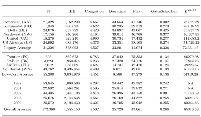
Tables 1a and 1b contain summary statistics, by carrier and year, for outcomes and inputs,
respec-tively.
We find starker differences among the carriers in the levels of inputs than in outcomes. On
average, low-cost carriers schedule half the downtime of their legacy competitors, with Southwest
responsible for the majority of this difference. Other low-cost carriers, which have more network
overlap with their legacy competitors and operate in the same large hubs (e.g., AirTran in Atlanta
Hartsfield), tend to schedule downtimes more similar to those of legacy carriers. Regarding
flexi-bility, low-cost carriers tend to schedule more aircraft of the same type to depart from an airport
in the same time block and day of week, despite operating at airports that are smaller on average.
We find that low-cost carriers tend to use gates much more intensively, i.e., they have a lower
ratio of gates to scheduled departures. Yet the carrier-specific averages reported in Table 1b mask
important variation in utilization. Figure 1 gives the mean of GatesSchedDepijt by carrier type and time of day. Peak is defined as the middle two 4-hour time blocks, while off peak includes the
first and last time block. Legacy carriers use gates less intensively at all times, but experience a
much greater change in gate utilization during peak hours.
The difference in the average per-month price paid by legacy and low-cost carriers to lease a
gate,pgates, is almost entirely due to low-cost carriers disproportionately serving the least expensive airports, e.g., Phoenix and Dallas Love Field, while legacy carriers disproportionately serve the
16
most expensive airports, e.g., San Francisco, Miami, Newark, and LaGuardia. Table 1b also shows
that low-cost carriers, particularly JetBlue and Southwest, tend to concentrate their operations in
less congested yet more concentrated airports, which gives them tremendous flexibility to shuffle
departures across gates to minimize delays.
Tables 1a and 1b also provide summary statistics by year. Interestingly, with the exception
of LoadF actor, there are no consistent trends in outcomes over time. LoadF actor has generally increased from 1997 to 2007, and then leveled out, while delays of all types appear to have reached
a peak in 2007 and subsided over the next two years. The descriptive statistics provide little
evidence of any shift in the intensity with which different operational inputs have been used over
time. However, airport concentration has risen substantially during this period.
Collectively, the carrier-specific summary statistics convey the importance of controlling for all
the factors that affect firms’ decisions about the levels of different operational inputs to employ in
a particular environment. This motivates our fixed-effects econometric approach in Section 3.2.
3
Econometric Specification of Directional Distance Function
The productivity literature in economics has recently developed theoretical and econometric tools
to characterize efficient operating practices in complex environments where firms convert multiple
inputs (Downtime, F lex, and GatesSchedDep) into multiple good outcomes (LoadF actor and
Cargo) and bad outcomes (P(> 15), P(> 60), and P(> 180)). Specifically, an output-oriented directional distance function characterizes the attainable set of outcomes for any given level of
inputs.17
3.1 Theoretical Properties of Directional Distance Function
Consider an airline production technology by which firms combine multiple operational inputs,
x = (x1, . . . , xN) ∈ RN+, to produce multiple good outcomes, y = (y1, . . . , yM) ∈ RM+, and bad
outcomes,ye= (˜y1, . . . ,y˜L)∈RL+. The firm’s production technology,P(x,y,ey), can be written as
P(x,y,ye) ={(x, y,y˜) :x can producey and ˜y}, (1)
whereP(x,y,ye) consists of all feasible input and outcome vectors.
17
Following Chambers et al. (1998) and F¨are et al. (2005), we define the output-oriented
direc-tional distance function as
− →
D(x,y,ye,gy,−gye) =β∗ = sup β
{β: (y+βgy,y˜−βgy˜)∈P(x,y,ey)}. (2)
The output-oriented directional distance function, →−D(x,y,ye,gy,−gey) provides a measure of the increase in good outcomes and decrease in bad outcomes needed to move a carrier to the frontier
of the production set,P(x,y,ye), for a given level of inputs. Thus, a carrier’sdistance is the scalar multiple of the direction vector, (gy = 1,−gey = 1), required to reach the production frontier.
As discussed in Chambers et al. (1998), the output-oriented directional distance function,
− →
D(x,y,ye,gy,−gey), defined in Equation 2 must satisfy the following properties to serve as a rea-sonable model of a firm’s production technology:
Non-Negativity:
− →
D(x,y,ye,gy,−gey)≥0 ⇐⇒ (y,y˜)∈P(x,y,ye). (P1)
Property P1 requires that the output-oriented directional distance function be non-negative,
with the most efficient firm having →−D(x,y,ye,gy,−gey) = 0. We ensure this property is satisfied via a normalization of the fitted function.
Translation Property:
− →
D(x,y+αgy,ye−αgey,gy,−gey) =
− →
D(x,y,ye,gy,−gey)−α. (P2)
Property P2 is true by definition of the output-oriented directional distance function, Equation
2. This property implies that increasingyand decreasing ˜y byα, multiplied by their respective directions, (gy = 1,−gey = 1), holding inputs constant, will result in a decrease in the output directional distance by α, and therefore an increase in efficiency equal to α. We ensure that Property P2 is satisfied via the parametric restrictions imposed during estimation and described
in Section 3.2.
g-Homogeneity of Degree Minus One:
− →
D(x,y,ye, λgy,−λgye) =λ−1
− →
D(x,y,ey,gy,−gye), λ >0. (P3)
Property P3 also follows directly from Equation 2, since scaling each element of the direction
gy and gy˜ by λ dividesβ∗ by λ.18 Property P3 is satisfied once P2 is imposed (via parametric
restrictions) and the model is estimated as described in Section 3.2.19
Good Outcome Monotonicity:
y′ ≥y→−→D(x,y′,ey,gy,−gye)≤
− →
D(x,y,ye,gy,−gye). (P4a)
and
Bad Outcome Monotonicity
e
y′ ≥ye→−→D(x,y,ye′,gy,−gye)≥
− →
D(x,y,ye,gy,−gye). (P4b)
Properties P4a and P4b state that the output-oriented directional distance function is
monoton-ically decreasing in good outcomes, while it is monotonmonoton-ically increasing in bad outcomes. That
is, holding all else constant, increasing a good outcome (or decreasing a bad outcome) moves the
directional distance function closer to zero, i.e., the carrier becomes more efficient. We test for
Properties P4a and P4b in Section 4 and find that they are satisfied, so that we do not need to
impose them during estimation.20
3.2 Econometric Methodology
The empirical specification of the directional distance function must capture the differences in the
operating models of low-cost and legacy carriers, control for sources of endogeneity, and satisfy
Properties P1-P4b. To accomplish this, we specify the directional distance function as
0 =−→D(xijkt,yijkt,yeijkt,wit,dijkt;gy,−gey, γ, φ, η) +εijkt, (3)
where
− →
D(xijkt,yijkt,yeijkt,wit,dijkt;gy,−gye, γ, φ, η)
= + N X
n=1
(γxn+φnxdLeg)xnijkt+ M X
m=1
γym+φmy dLeg
yijktm + L X
l=1
γyle+φlyedLeg
e
ylijkt (4)
+ (γw+φwdLeg)wit+ γienvir+φenviri dLeg
denviri
+ηaircraf tk daircraf tk +ηtyr−mondyrt −mon+ηrreg−mondrreg−mon+ηjcarrierdcarrierj
18
By normalizing all outputs to be unit-free prior to estimation, we make the distance function estimates unit free. Following estimation, we can then convert back to the original units for our analysis.
19
These parametric restrictions are analogous to imposing linear homogeneity when estimating a cost function (e.g., Equation 2 in Berndt and Wood 1975).
20
and
εijkt=υijkt−uijkt. (5)
Following F¨are et al. (2005), the left-hand side of Equation 4 is set equal to zero, representing
frontier production (i.e., fitteddistance of zero).
The functional form of Equation 4 permits differences in the operating models of low-cost and
legacy carriers through the interaction of a legacy indicator,dLeg, with the vector of good outcomes, y, comprised of LoadF actorijt and Cargoijt, the vector of bad outcomes, ye, comprised of P(> 15)ijkt,P(>60)ijkt, andP(>180)ijkt, the vector of inputs,x, comprised ofF lexijkt,Downtimeijkt, andGatesSchedDepijt, and a vector of time-varying factors that impact a carrier’s ability to convert inputs to outcomes,w, comprised ofCongestionit andHHIit.
To capture as many sources of endogeneity as possible, including unobserved determinants of
carriers’ input choices and outcomes, as well as unobserved inputs, by including fixed effects for an
aircraft’s crew-rating (daircraf tk ), each year-month (dtyr−mon), each region-month (dregr −mon), each carrier (dcarrier
r ), and each environment for each carrier type (interaction ofdLeg anddenviri indica-tors). The aircraft crew-rating fixed effects control for larger aircraft requiring greater downtime,
as well as unobserved inputs like the number of flight attendants and pilots, which are mandated by
the FAA. The year-month fixed effects control for any temporal industry-wide shocks that impact
productivity, like the events of September 11th and its lingering effects (e.g., additional security
procedures and diminished demand). The region-month fixed effects control for differential weather
patterns across regions. The carrier fixed effects control for time-invariant carrier-specific factors
and the average effect of time-varying carrier-specific factors, such as wage differentials and carrier
size. The carrier-type and environment-specific fixed effects control for time-invariant unobservables
specific to environmentifor low-cost and legacy carriers, respectively. Collectively, in addition to removing sources of endogeneity, these controls allow the frontier to be characterized by lower levels
of good outcomes and higher levels of bad outcomes from the same level of inputs, in more difficult
environments.
Following Atkinson and Primont (2002) and F¨are et al. (2005), we decompose the error term,
εijkt, into a one-sided component,uijkt>0,that captures unmeasured time-varying differences in carriers’ managerial ability or operational difficulties unique to specific carriers, and a two-sided
mean-zero idiosyncratic component,υijkt, that allows for random and transitory shocks impacting carriers’ ability to transform inputs to outcomes, such as poor weather. We make no parametric
Like F¨are et al. (2005), our parameter estimates are chosen to satisfy
{bγ,φ,b ηb}=arg min
{γ,φ,η} X
i,j,k,t
0−−→D(xijkt,yijkt,yeijkt,wit,dijkt;gy,−gey, γ, φ, η) 2
,
subject to
i) −→D(xijkt,yijkt,yeijkt,wit,dijkt;gy,−gey, γ, φ, η)≥0, for all (i,j,k,t)
ii) M P m=1
γm y gy−
L P
l=1
γl e
ygye=−1
iii) M P m=1
γm y +φmy
gy − L P l=1 γl e y+φlye
gye=−1
iv) ∂
− →
D(xijkt,yijkt,yeijkt,wit,dijkt;gy,−gey,γ,φ,η)
∂yem ≥0.
v) ∂
− →
D(xijkt,yijkt,eyijkt,wit,dijkt;gy,−gye,γ,φ,η)
∂ym ≤0
The estimated parameters, {bγ,φ,b ηb}, make the carriers look as efficient (i.e., fitted distance as close to zero) as possible while satisfying properties i)-v).21 Constraint i) ensures Property P1, non-negativity, is satisfied. We ensure that i) holds via a normalization of the estimated distance
function, increasing all fitted distances by the absolute value of the most negative fitted distance.
Constraints ii) and iii) ensure that the translation property and g-homogeneity are satisfied for
legacy and low-cost carriers, respectively. These constraints are imposed parametrically during
estimation. Constraintsiv) andv) ensure Properties P4a and P4b, monotonicity, hold. We do not
imposeiv) or iv), since we find the unconstrained solution satisfies monotonicity.22
The stochastic directional distance approach is very similar to well-studied non-stochastic
linear-programming solutions, but also different in important ways. Specifically, if our objective function
were an absolute rather than quadratic loss function, the problem would reduce to a linear program
similar to the non-stochastic optimization specification of F¨are et al. (2005). For our purposes, a
stochastic approach is preferable for two main reasons. First, the non-stochastic problem does not
allow for random shocks to productivity, the υijkt term in Equation 5, which is important for our problem. Airlines face a number of events outside their control (e.g., 9/11, airport-specific opera-tions, severe weather, etc.), that should not be reflected in any calculation of productivity. Thus,
21
Rather than estimate over 4,000 unique coefficients corresponding to the carrier-type and environment specific fixed effects, we follow an algebraically equivalent procedure and difference the distance function prior to estimating the remaining parameters.
22
our calculation of technical inefficiency is based solely onuijkt. Second, we are particularly inter-ested in comparing the statistical significance of the returns to various robust-scheduling practices,
which requires that we employ a stochastic model.
3.3 Visualization of Directional Distance Function Approach
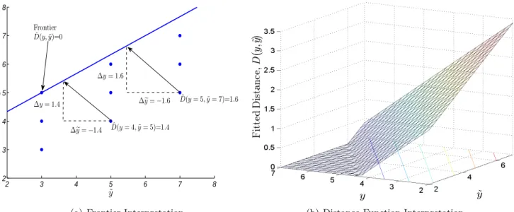
Below, we use a simple example to illustrate the mechanics of the directional distance function
approach and how it characterizes a frontier corresponding to efficient production. Assume that
there is one good outcome,y, and one bad outcome, ˜y, and that our data consist of carriers (of the same type) that employ the same amount of an input,x. In this case, the econometric objective function is
{ϕc0,ϕc1,ϕc2}=arg min
ϕ0,ϕ1,ϕ2
X
r
(0−ϕ0−ϕ1yer−ϕ2yr)2, (6)
subject to
i) ϕ0+ϕ1yer+ϕ2yr≥0, for all r
ii-iii) ϕ2−ϕ1 =−1
iv-v) ϕ1 ≥0 andϕ2 ≤0
Constraint i) ensures non-negativity, ii) and iii) reduce to one constraint (as there is only one
carrier type), which ensures that the translation property and g-homogeneity are satisfied. The
monotonicity restrictions are iv)-v). The objective is to identify parameter values that make the
carriers look as efficient as possible – i.e., minimize fitted distance – while satisfying the constraints
that impose properties necessary to have a well-defined production technology. The most efficient
carriers have a fitted distance of zero.
The example data, nine ordered pairs indexed byr, are plotted in Figure 2(a). Figure 2(b) plots the fitted distance function,cϕ0−ϕc1ye−ϕc2y(normalized to be non-zero) through the sample points,
along with the level sets of the plane. Note that the fitted distance is strictly increasing (decreasing)
in the bad (good) outcome (i.e., monotonicity), and all fitted distances are strictly positive, while
satisfying ϕ2−ϕ1 =−1. The level sets of the distance function are useful, because the level set
corresponding to a fitted distance of zero characterizes the tradeoffs between outcomes faced by an
efficient carrier. This tradeoffs can also be seen as a traditional production frontier, plotted in Figure
2(a), by re-arranging the fitted distance function, asy=−cϕ0
c ϕ2−
c ϕ1
c
2 3 4 5 6 7 8 2
3 4 5 6 7 8
˜ y
y ˆ
D(y= 5,˜y= 7)=1.6
∆y= 1.6
ˆ
D(y= 4,y˜= 5)=1.4
∆y= 1.4
∆ye=−1.4
∆ey=−1.6
Frontier ˆ
D(y,˜y)=0
(a) Frontier Interpretation (b) Distance Function Interpretation
Figure 2: Visualization of Directional Distance Function Approach
of this frontier,−ϕc1
c
ϕ2, which would also be obtained by implicitly differentiating the fitted distance
function directly. From the definition of the directional distance function, Equation 2, the fitted
distances can be visualized as the scalar multiple of the direction vector, (gy = 1,−gy˜= 1), required
to reach the production frontier by moving horizontally and vertically as defined in Equation 2 and
indicated in Figure 2(a) with the dotted lines.
One can also easily visualize our measures of technical efficiency, which we discuss in Section
4.5, using Figure 2(a). For example, our measure of technical efficiency for the good outcome is the
maximum additional amount of the good outcome that is feasible given the levels of other outcomes
and inputs, i.e., the vertical distance from one of the points in Figure 2(a) to the frontier. The
measure of technical efficiency for the bad outcome is the horizontal distance to the frontier.
4
Results
Figure 3 provides a guide for the discussion below. We first discuss the coefficient estimates of
the directional distance function in Section 4.1. In Section 4.2 we describe how these estimates,
together with gate-price data, enable us to obtain the per-unit cost of the other inputs. Next,
in Section 4.3, we demonstrate how to use the coefficient estimates from Section 4.1 and cost
estimates from Section 4.2 to obtain the per-unit and per-dollar returns for each outcome from
Figure 3: Overview of Results Discussion
and estimates of passenger and cargo own-price demand elasticities, to estimate the passenger and
cargo revenues earned per dollar spent on each robust-scheduling input. In section 4.4 we use the
coefficient estimates from Section 4.1 to analyze tradeoffs between outcomes, and then combine
these estimated tradeoffs with data on ticket prices to uncover the value to carriers from reducing
delays of different lengths. In Section 4.5 we estimate carriers’ technical efficiencies and use these
to identify avenues for operational improvement and predict the increase in profitability from these
improvements.
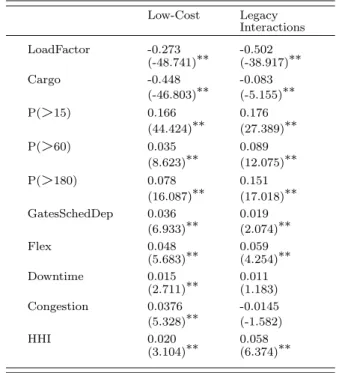
4.1 Estimates of Directional Distance Function Coefficients
Table 2 contains the estimates of Equation 4.23 Columns 1 and 2 of Table 2 report the coefficient estimates for low-cost carriers and the interaction of each variable with the legacy-carrier indicator,
dLeg, respectively. All coefficients in Table 2 are statistically significant, except for two interactions with the legacy-carrier indicator. This lack of significance for the congestion interaction is not
surprising, as congestion should not affect carriers differentially. Thus the grouping of carriers into
low-cost and legacy types separates out important sources of systematic heterogeneity among the
carriers while using a computationally feasible number of parameters.
The coefficient estimates in Table 2 have a straightforward interpretation, as discussed in Section
3.2. For example, the positive coefficient on GatesSchedDep implies that holding constant other
23
inputs and outcomes, an increase in GatesSchedDep corresponds to a greater distance from the frontier. In other words, a carrier is regarded as less efficient if it achieves the same outcomes
while using gates less intensively. The coefficients for other inputs can be interpreted similarly.
For good (bad) outcomes, one expects a negative (positive) coefficient such that an increase in the
outcome holding all other outcomes and inputs constant results in a lesser (greater) distance from
the frontier. Our estimates yield the expected sign for each outcome. Thus, Properties P4a and
P4b are satisfied despite not being imposed during estimation.
The positive sign on HHI is consistent with prior work (see Mayer and Sinai 2003), which suggests that the frequency of delays should be inversely related to concentration, since carriers
have a greater incentive to internalize the effect of their actions in more-concentrated environments.
Thus the minimum attainable level of delays is lower in more concentrated environments.
4.2 Estimates of Input Costs
The use of robust-scheduling inputs generates both direct and indirect costs. For example, an
additional minute of scheduled downtime directly increases costs due to lost revenue, but indirectly
reduces costs due to increased connectivity. Since legacy carriers operate hub-and-spoke networks,
we expect this benefit to substantially lower their costs of downtime. Similarly, altering aircraft
routings to increase flexibility by ensuring that more aircraft of the same type depart at similar
times can affect connection opportunities and the desirability of flight departure times.
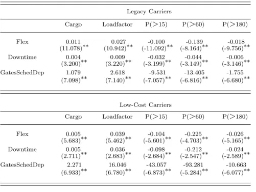
To estimate the costs of robust-scheduling inputs, we first estimate the tradeoffs between these
inputs, which we combine with gate price data to infer the costs of the other inputs. Since a
frontier firm has a fitted distance of zero, −→D(xijkt,yijkt,yeijkt,wit,dijkt;gy,−gye,γ,b φ,b ηb) = 0, by the implicit function theorem, the rate at which such a carrier can trade off between inputsxnand
xn′
, while holding outcomes constant, is
dxn
dxn′ =−
∂−→D ∂xn′
∂−→D ∂xn
. (7)
Table 3 contains our estimates of these tradeoffs, which are themselves of interest. For example, we
find that, at the margin, a legacy carrier can reduce scheduled downtime on each flight by about
3.13 minutes and keep outcomes constant if one more flight of the same aircraft type is scheduled to
depart in the same time block (i.e., if flexibility is increased by one unit), in contrast to a reduction
of only 1.06 minutes for low-cost carriers.
0 5 10 15 20 25 30 0
0.1 0.2 0.3 0.4 0.5 0.6 0.7 0.8 0.9 1
Minutes
CDF
Off−Peak
Peak
(a) Legacy
0 5 10 15 20 25 30
0 0.1 0.2 0.3 0.4 0.5 0.6 0.7 0.8 0.9 1
Minutes
CDF
Off−Peak
Peak
(b) Low Cost
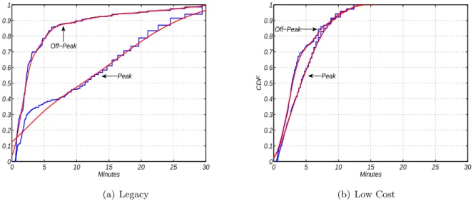
Figure 4: CDF of Per-Flight Downtime (Minutes) Equivalent to Additional Gate
downtime on each flight must be increased to keep outcomes constant if a carrier had access to
one less gate, during peak and off-peak hours, for legacy and low-cost carriers respectively. These
distributions arise for each carrier type because of how the return to a gate varies with each
environment, which we characterize as a combination of airport, time-of-day and day-of-week.24 In environments where a carrier is using gates intensively, the loss of a gate can be offset only by a
large increase in downtime. Notice that these results are consistent with Figure 1. Legacy carriers
have a greater change in gate utilization during peak than low-cost carriers, resulting in a larger
difference in how much downtime must be added during peak and off-peak hours to offset losing a
gate. We perform a similar calculation to recover the increase in flexibility needed to offset losing
a gate and find that low-cost carriers require a much larger increase in flexibility to hold outputs
fixed.
Next, we combine the estimates in Table 3 with gate-price data to infer the costs associated
with each robust-scheduling input. Knowing the tradeoffs faced by a carrier seeking to achieve a
given level of outcomes at least cost, along with the price of one input, one can infer the costs of
all other inputs. Specifically, to minimize the cost of obtaining any set of outcomes, the marginal
productivity per dollar for each pair of inputs, xn and xn′
, must be equal to the ratio of their
24
Note that our estimates relate the fitted distance to GatesShedDep, not Gates. Thus the relationship between the fitted distance and Gates is a nonlinear function of SchedDep, ∂−→D
∂Gates=
∂−→D ∂GatesSchedDep
1
0 10 20 30 40 50 60 70 80 0 0.1 0.2 0.3 0.4 0.5 0.6 0.7 0.8 0.9 1 Dollars CDF (a) Legacy
0 10 20 30 40 50 60 70 80
0 0.1 0.2 0.3 0.4 0.5 0.6 0.7 0.8 0.9 1 Dollars CDF
(b) Low Cost
Figure 5: CDF of Per-Minute Downtime Costs by Carrier Type
respective prices,pn and pn′
,
dxn
dxn′ =−
∂−→D−
∂xn′
∂−→D−
∂xn
= p
n
pn′. (8)
For example, our estimates provide the additional minutes of scheduled downtime required to
keep outcomes constant if a carrier operating on the frontier had one less gate. Since we know
the actual cost of a gate at each airport,GateP rice, we can use Equation 8 to infer how a carrier perceives the per-minute cost of downtime. Figures 5(a) and 5(b) give the distribution of the
calculated per-minute cost of downtime for legacy and low-cost carriers, respectively. These results
rationalize low-cost carriers scheduling approximately half as much downtime as legacy carriers, as
the median per-minute cost of downtime for low-cost carriers is $17.83 versus only $9.32 for legacy carriers. Direct measures of these operating costs would understate this difference, as the higher-fare
legacy carriers may actually forgo more revenue from downtime. Instead, our cost estimates also
incorporate indirect opportunity costs, which include the benefits of increased network connectivity,
that are greater for legacy carriers operating hub-and-spoke networks.25
Performing a similar calculation using Equation 8 for flexibility, we find that this input is much
more costly for legacy carriers. The median cost to a legacy carrier of increasing flexibility by
25
scheduling one additional flight of a given aircraft type to depart in a particular time block is
over $900, versus a median of just under $200 for low-cost carriers. This differential is consistent
with low-cost carriers focusing on high-density routes and operating more homogenous fleets, as
well as having a less complex scheduling problem than legacy carriers, which must maintain a
high degree of connectivity throughout their network, further increasing the opportunity cost of
flexibility. The lower cost of flexibility enjoyed by low-cost carriers does come with greater risk, such
as increased vulnerability to problems that might arise with a particular aircraft or engine type.
These include design defects, mechanical problems, contractual performance by the manufacturers,
or public perception regarding the safety of the aircraft.
Note that the input costs we identify are derived based on the assumption that airlines achieve
the observed level of outcomes in the least-cost way, given their operating model. Since our estimates
of the costs of robust-scheduling inputs can explain actual differences in the scheduling patterns
of carriers, we conclude that carriers appear to be selecting the least-cost means of producing
outcomes.
4.3 Estimates of Returns to Inputs
We first use our estimates of the directional distance function coefficients to identify the unit return
for each outcome per unit of each input. Specifically, the rate at which a good outcome,ym, changes in response to an input,xn, for an efficient carrier is given by the implicit function theorem,
dym dxn =−
∂
− →
D−
∂xn
∂−→D−
∂ym
. (9)
We use a similar calculation for each bad outcome,eyl. For each outcome, Table 4 reports estimates of the mean return per unit of input, with associated t-statistics. Note that the estimates all
have the expected signs – inputs increase good outcomes and decrease bad outcomes – and are
statistically significant. We find that per-unit returns for most of the inputs are greater for
low-cost carriers. This is consistent with low-low-cost carriers employing more homogenous fleets, operating
on tighter schedules, and using boarding gates more intensely. Interestingly, we find that for every
outcome, the per-unit returns to gates per scheduled departure are significantly greater than for
the other two inputs.
Next, we examine whether this pattern persists after controlling for the cost of each input. We
estimate the improvement in each of the outcomes for each dollar spent on an input, by combining
average improvement in outcomes per $1,000 spent on the our three inputs for both carrier types.
Formally, this is accomplished by dividing Equation 9 by the per-unit price of the input (xn),pn, and multiplying by 1,000.
Consider an investment in gates by a low-cost carrier of $1,000 per flight.26 From the bottom
row of Table 5, this investment results in an improvement of 6.87% (1.23/17.9) in the proportion
of flights 15 or more minutes late,27 which is substantially greater than the 4.30% (0.77/17.9)
reduction from flexibility or 1.96% (0.35/17.9) reduction from downtime, and this difference is
statistically significant. For the low-cost carrier investing in gates, in addition to improved
on-time performance, the attainable levels of cargo and loadfactor also increase, and the frequency of
long delays is reduced. For legacy carriers, a $1,000 investment in gates yields the greatest relative
improvement, although this effect is about one-fourth that achieved by low-cost carriers. This result
is consistent with legacy carriers’ heterogenous fleets, longer downtimes, and less intensive use of
gates. Thus Table 5 reveals that the most cost-effective way for a carrier to target improvement
along any outcome dimension is by better managing gates for greater recovery robustness. Yet
gates management has received almost no attention in the OR scheduling literature (Barnhart et
al. 2003).
From a public-policy standpoint, the substantial differences in returns to gates between carrier
types suggest that the greatest improvements in consumer welfare from reduced delays can be
realized by assigning additional gate capacity to low-cost carriers. This result complements a
growing literature on the role that airports have in determining equilibrium outcomes and passenger
welfare through gate-leasing practices (e.g., Ciliberto and Williams 2010, Snider and Williams 2014).
The average returns reported in Table 5 mask substantial heterogeneity and do not reveal the
revenues that result from changes to scheduling inputs. To demonstrate this, Figures 6(a)-6(c)
report, by carrier type, the smoothed probability distribution functions of the increase in passenger
and cargo revenues per flight, per $1,000 spent on each input. We calculate this additional revenue
accounting for the negative tradeoff between loadfactor and ticket prices, and between cargo volume
and its price. Specifically, for passenger revenues, we use route-specific price-elasticities of demand
from the survey of empirical estimates in IATA (2008), which enables us to account for variation
in the mix of routes (long-haul vs. short-haul) served by each carrier. We draw our estimates
of the own-price elasticity for cargo from the survey of empirical estimates in Hellerman (2006).28
26
To be comparable across the different inputs, the size of the investments must be normalized this way, since gates impact all flights, flexibility a subset of flights, and downtime a single flight.
27
From Table 1a, 17.9% is the average frequency of flights over 15 minutes late for low-cost carriers.
28
(a) Downtime (b) Flex (c) Gates
Figure 6: PDFs of Total Passenger and Cargo Revenues Per $1,000 Spent on Inputs
With these elasticity estimates, the rate of change in total revenues from passengers and cargo from
increasing an input,xn, is given by
M X
m=1
d[pmym]
dxn = M X
m=1
dym
dxn
pm+dp m
dymy m
=
M X
m=1
∂
− →
D ∂xn
∂−→D ∂ym
pm
1 + 1
ǫm
, (10)
wherepm andǫm are the prices and own-price elasticity of demand for the respective outcomes.29
Figures 6(a), 6(b), and 6(c) report the revenue increase from a $1,000 expenditure on Downtime,
Flex, and Gates, respectively. Legacy carriers generate substantially less revenues from expenditure
on each of the inputs. Consistent with Table 5, increased expenditure on gates generates the greatest
revenues. The multi-modal distributions of returns to gates arise for two reasons: differences in
utilization across the day and differences in the leasing costs across airports. For both carrier
types, there are substantial differences in the returns to boarding gates during peak and off-peak
hours. Even though low-cost carriers maintain more consistent use of gates throughout the day,
the intensity of use is so much greater at all times that slight differences in utilization over the day
results in substantial variation in returns.
for short-haul routes. The median cargo own-price elasticity of demand is -1.3. We use the median estimate for each demand elasticity in our calculations, permitting the passenger elasticity to vary depending on the route distance, a major determinant of the availability of reasonable substitutes for air travel.
29
4.4 Estimates of Tradeoffs between Outcomes
While airlines can improve particular operational outcomes by investing in robust-scheduling
in-puts, they can instead improve some outcomes by sacrificing performance on other outcomes. Our
estimated production frontier determines the decline along one outcome dimension necessitated by
an improvement along another, if inputs are held constant (Porter 1996, Lapre and Scudder 2004).
The tradeoffs carriers are willing to make depend on the value they place on each outcome.
As in Section 4.3, our estimates of the directional distance function can be used to quantitatively
measure these tradeoffs. For any two good outcomes,ym andym′
, an efficient carrier can trade off
along the frontier between any two outcomes at the rate
dym
dym′ =−
∂−→D ∂ym′
∂−→D ∂ym
. (11)
The set of such tradeoffs for each pair of outcomes is presented in Table 6, by carrier-type. For both
types of carriers, our estimates satisfy a null-jointness condition, despite not imposing this during
estimation. That is, carriers cannot increase a good outcome (LoadF actor or Cargo) without an associated increase in a bad outcome (P(>15), P(>60), or P(>180)), for any level of inputs.
Our estimates in Table 6 enable us to analyze the tradeoffs between outcomes and develop useful
managerial insights. For example, we find that a legacy (low-cost) carrier may trade off an increase
of 1% inP(>15), poorer on-time performance, for a 0.31% (0.38%) increase inLoadF actor.30 Using a calculation similar to Equation 10, for each carrier type, we calculate the additional revenue gained
by increasingP(>15) by 1%.31 We find that legacy and low-cost carriers can increase revenues by $74.33 and $68.45 per flight, respectively, by accepting a 1% increase inP(>15). Such a tradeoff may be preferable to increasing expenditure on inputs (Table 5). To put this in perspective, for
Southwest Airlines in 2007 this amounted to about 0.8% of total revenues per flight, or $78 million
across their entire network (over 1.1 million flights). Additionally, we find that both types of
carriers value a 1% reduction in the probability of a flight delay lasting over 180 minutes at more
than 4 times as much as one lasting over 15 minutes. This result reinforces the finding of Ramdas
et al. (2013) that carriers’ market value is most strongly impacted by the frequency of long delays
(P(>180)). It also rationalizes Southwest’s strategy of swapping aircraft and crews to parse one long delay, possibly due to an aircraft incurring a mechanical failure, into many short delays.
30
Rupp (2009) also documents a tradeoff betweenLoadF actorand delays.
31
Our estimates of the value carriers place on delays can also guide regulatory policy, which must
balance the benefits to passengers of fewer delays against the costs to carriers of limiting the severity
and frequency of delays.32 Currently, as part of the FAA Modernization and Reform Act of 2012 (Section 406(b)), the DOT is conducting such a review of “carrier flight delays, cancelations, and
associated causes...”. This includes assessing “air carriers’ scheduling practices” and “capacity
benchmarks at the Nation’s busiest airports,” as well as providing “recommendations for programs
that could be implemented to address the impact of flight delays on air travelers.” Our estimates
give policy makers insight into the costs that carriers would incur if forced to amend scheduling
practices to reduce delays. These can then be weighed against the costs of alternative ways to
reduce delays, such as building additional airport facilities to alleviate congestion (Daniel 1995).
4.5 Operational Efficiency Measures
Following Agee et al. (2012), we now use our estimates of the directional distance function to
quantify each carrier’s technical efficiency, i.e., their ability to attain the efficient level of outcomes
from a given level of inputs, and then measure the impact on profits of any inefficiencies. Rather
than repeating each step of this calculation, our approach is most easily explained using our example
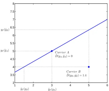
from Section 3.3.33 Consider two of the carriers from this example, A and B, which are labeled
in Figure 7. As before, there is one good outcome, y, and one bad outcome, ye, and the figure is drawn for a particular level of inputs, x. Carrier A is on the frontier, with a fitted distance of zero, while carrier B is technically inefficient, with a positive fitted distance. Our estimates of what
constitutesfrontier or efficient production enable us to quantify how much better the outcomes for
inefficient carriers can be. As shown in Figure 7, holding fixed the level of the good outcome for
carrier B, yB, this carrier can decrease the bad outcome by ˜yB−y˜F(yB). Similarly, holding fixed the bad outcome, ˜yB, carrier B can increase the good outcome byyB−yF(˜yB). We use this idea of a shortfall fromfrontier production to calculate our measures of technical efficiency.
In our data, we observe each carrier, j, operating different aircraft,k, in various environments,
i, over a long period of time. In addition, we have multiple good and bad outcomes. As a result, we calculate a carrier’s j′s average technical efficiency for each good outcome, ym, over different aircraft,k, and environments,i, in which they operate in each year,t, as
32
Recent work in economics, Snider and Williams (2014), suggests that current federal policy which limits airports’ ability to raise capital to expand airport facilities both limits competition and worsens the frequency and length of delays.
33
1 2 3 4 5 6 3
3.5 4 4.5 5 5.5 6 6.5 7 7.5 8
C arrier A
ˆ
D(yA,y˜A) = 0
C arrier B
ˆ
D(yB,y˜B) = 1.4
yF(˜yB)
yF(˜yA)
˜
yF(yB) y˜F(yA)
Figure 7: Technical Efficiency Measures
T Ejtym = 1
Njt X
i,k
yijktm ymF
ikt (y− m
ijkt,yeijkt,xijkt)
,
where
yiktmF(xijkt,yijkt−m,yeijkt) = sup{yn:
− →
D(xijkt,yijkt,yeijkt,wit,dijkt;gy,−gey,γ,b φ,b ηb)≥0},
y−ijktm is the vector of other good outcomes (i.e., besides yn) produced by carrier j, andN
jt is the
number of observations for carrierj in periodt. Our measure of technical efficiency for each good outcome is thus the average percentage shortfall from the relevant frontier outcome level across
those environments in which the carrier operates in periodt. Similarly, for a bad outcome, yel, we measure each carrier’s operational efficiency as
T Ejteyl = 1− 1
Njt X
i,k h
e
yijktl −eylFikt(yijkt,ye−ijktl ,xijkt) i
,
where
e
yiktlF(yijkt,yeijkt−l ,xijkt) = inf{yel:
− →
D(xijkt,yijkt,yeijkt,wit,dijkt;gy,−gey,γ,b φ,b ηb)≥0}
andyeijkt−l is the vector of other bad outcomes (i.e., besides eyl) produced by carrier j.
The reason for taking the difference of a carrier’s outcome and thefrontier outcome level in the
case of bad outcomes (i.e., our delays measures) is that the frontier firm might have zero delays so
respect to each of the bad outcomes is the reduction in the bad outcome that would be required
to reach the frontier, holding constant inputs and other outcomes. This bounds our measures of
technical efficiency for both good and bad outcomes between zero and one.34
In Table 7, we report the estimates of carriers’ average efficiency in 2007, and, since we have
actual prices for the two good outcomes, cargo and loadfactor, we also report lost revenue due
to the inefficient production of these outcomes.35 Similar to our analysis of returns to inputs in
Equation 10 of Section 4.2, we utilize the elasticity of demand for cargo and passengers to calculate
the tradeoff between volume and price.
For good and bad outcomes, the relative measures are bounded between 0 and 1, with the most
efficient firm having a value of 1. For example, Delta’s relative measure of 0.91 for LoadF actor
(a good outcome) implies that, after conditioning on levels of inputs and other outcomes, Delta
achieves 91% of the frontier level of LoadF actor defined by American. By our estimates, Delta lost over $500 million in 2007 due to its load-factor inefficiencies, even after accounting for the
reduction in ticket price needed to achieve an efficient level of load factor. The results for cargo are
less dramatic, but still substantial, as Delta’s inefficiencies in this regard resulted in lost revenue
of over $21 million. Similarly, Delta’s technical efficiency measure of 0.98 for P(> 180) implies that Delta can increase profits by reducing the frequency of long delays by 0.02, with no additional expenditure on inputs.
The efficiency results in Table 7 for the delay measures demonstrate the value of our directional
distance function approach, which characterizes the efficient level for each of the multiple outcomes
for any given level of inputs and operating environment. Northwest is the most efficient carrier
for each of the delay measures; however, Continental is a very close second. Yet this result is
completely counter to Table 1a if one considers the delay measures in isolation, as Continental
performs rather poorly across each measure of delays. However, Continental employs much smaller
amounts of Downtime and F lex than other legacy carriers, and is very near the top in terms of gate utilization. Thus, once the level of all inputs, all outcomes, and the operating environment is
accounted for, Continental is relatively efficient. American’s last-place ranking for each of the bad
34
Note that our measures of efficiency credit carriers for operating in more difficult environments by normalizing their outcome levels by thefrontieroutcome level in each environment. In difficult environments, the frontier outcome level is characterized by higher levels of bad outcomes and lower levels of good outcomes. Thus, a carrier’s performance relative to the best practices in each environment is captured by our measures.
35