Within-Firm Pay Inequality
∗
Holger M. Mueller
†Paige P. Ouimet
‡Elena Simintzi
§November 2016
Abstract
Financial regulators and investors alike have expressed concerns about high pay
inequality within firms. Using a proprietary data set of public and private firms, this paper shows that firms with higher pay inequality–relative wage differentials between top- and bottom-level jobs–are larger and have higher valuations, better
operating performance, and higher equity returns. High-inequalityfirms also exhibit larger earnings surprises, consistent with the argument that pay inequality is not
fully priced by the market. Overall, our results support the notion that high pay
disparities withinfirms are a reflection of better managerial talent.
∗We thank David Autor, Xavier Gabaix, Xavier Giroud, Claudia Goldin, Johannes Stroebel, and
seminar participants at MIT, NYU, and the 2015 Labor and Finance Group conference for valuable comments. We are grateful to Raymond Story at Income Data Services (IDS) for help with the data.
1
Introduction
Rising income inequality has garnered attention in the media and among policy circles.1
The argument in the public domain is that inequality may be harmful for economic growth
(Persson and Tabellini (1994), Alesina and Rodrik (1994), Easterly (2007), IMF (2014)),
impair intergenerational mobility (OECD (2011), Corak (2013)), and even cause deep
financial and real crises, such as the Great Depression or the Great Recession (Rajan
(2010), Kumhof, Rancière, and Winant (2015)).
Interest in pay inequality extends beyond macroeconomics. Financial regulators and
investors alike have recently expressed concerns about high pay inequality within firms:
“High pay disparities inside a company can hurt employee morale and productivity, and
have a negative impact on a company’s overall performance” (Julie Fox Gorte, PAX
World Management (2013)). In agreement, the Securities and Exchange Commission, as
mandated by Section 953(b) of the Dodd-Frank Act, has adopted a new rule requiring
companies to disclose theratio of median employee pay to that of the chief executive offi
-cer.2 Market participants have reacted positively to this pay ratio disclosure: “Grosvenor
believes that income inequality and a shrinking middle class are real and important issues
that our country needs to address. We believe transparency and disclosure such as that
called for in the proposal, which disclose a “pay ratio,” can be helpful in allowing investors
to more accurately judge the effect of pay structure on company performance” (Michael
J. Sacks, Grosvenor Capital Management (2013)).3
This study examines how pay inequality varies across firms, how it relates to firms’
operating performance and valuations, and whether it is priced by the market. From a
1See, for instance, Alan Krueger’s (2012) speech as Chairman of the Council of Economic Advisers
on the “The Rise and Consequences of Inequality,” as well as debates in the media and academic circles ignited by Thomas Piketty’s (2014) book “Capital in the Twenty-First Century.”
2The rule is effective October 17, 2015. Firms must comply by thefiscal year beginning on or after
January 1, 2017. The pay ratio disclosure applies to allfirms except emerging growth companies, smaller reporting companies, and foreign private issuers.
3Similarly, Anne Simpson (2013) from CalPERS concludes: “We believe that pay ratio disclosure,
required by Section 953(b) of Dodd-Frank, will provide important supplementary information on the
theoretical perspective, pay inequality may vary across firms for a number of reasons.4
It could, for example, reflect differences in managerial talent, provision of incentives, or
managerial rent extraction. While our main results are consistent with pay inequality
being a reflection of managerial talent or incentive provision, they are inconsistent with
rent extraction. Additional tests suggest that managerial talent is a key driver of pay
disparities within firms.
Empirical investigation of pay inequality within firms is challenging due to lack of
publicly available data. To address this challenge, we employ a proprietary data set
of UK firms in which employee pay is observed at the firm-job title-year level. Job
titles are grouped into nine hierarchy levels, allowing us to measure how pay disparities
between hierarchy levels vary across firms. For instance, level 1, our lowest hierarchy
level, includes work that “requires basic literacy and numeracy skills and the ability
to perform a few straightforward and short-term tasks to instructions under immediate
supervision.” Typical job titles are cleaner, labourer, and unskilled worker. Level 5, in
the middle of the hierarchy, includes work that “requires a vocational qualification and
sufficient relevant specialist experience to be able to manage a section or operate with
self-contained expertise in a specialist discipline or activity.” Typical job titles are engineer,
marketing junior manager, and warehouse supervisor. And level 9, the highest hierarchy
level, includes “very senior executive roles with substantial experience in, and leadership
of, a specialist function, including some input to the organisation’s overall strategy.”
Typical job titles arefinance director, HR director, and lawyer/head of legal.
To obtain measures of within-firm pay inequality, we construct pay ratios comparing
the pay across different hierarchy levels within the samefirm and year. For example, “pay
ratio 19” compares the pay of top-level executives, such asfinance and HR directors, with
the pay of unskilled workers or cleaners at the bottom of the firm’s hierarchy. There are
nine hierarchy levels, leaving us with(9×8)2 = 36 pay ratios.
We find that larger firms exhibit significantly more pay inequality. This result is
4As in the macro- and labor economics literature, we refer to pay inequality as the disparity in pay
entirely driven by hierarchy levels where managerial talent is important (levels 6 to 9).
By contrast, pay ratios comparing lower hierarchy levels to one another (levels 1 to 5)
are largely invariant with respect tofirm size. Accordingly, an HR director’s pay (level 9)
increases relative to the pay of an unskilled worker (level 1) asfirm size increases. However,
the pay of an ordinary HR/Personnel officer (level 4) does not increase relative to the pay
of an unskilled worker. The effect of firm size on pay inequality is economically large.
Moving from the 25th to the 75th percentile of the firm-size distribution–an increase in
firm size of 1,565%–raises the pay associated with hierarchy level 9 by 280.1% relative
to the pay associated with hierarchy level 1. By comparison, the pay associated with
hierarchy level 6 increases only by 59.7% relative to the pay associated with hierarchy
level 1. Consequently, an increase in firm size has a roughly five times bigger impact on
pay ratio 19 than it has on pay ratio 16.
While firm size plays a key role for theories emphasizing the efficient assignment of
managerial talent, our size results are also potentially consistent with either incentive
provision or rent extraction. To distinguish between rent extraction and the other two
hypotheses, we examine how pay inequality is related tofirms’ operating performance and
valuations. If pay inequality is primarily a reflection of managerial talent or the provision
of incentives, we would expect firms with more inequality to have better operating
per-formance and higher valuations. By contrast, if pay inequality is merely a reflection of
managerial rent extraction, we would expect firms with more inequality to exhibit worse
operating performance and lower valuations. Regardless of whether we consider thefirm’s
return on assets or Tobin’s Q, we find that high-inequality firms are better performers
and have higher valuations.
In additional tests, we seek to distinguish between talent assignment and incentive
provision. The underlying idea is that if moral hazard is the key channel, we should see
stronger results in environments where moral hazard is potentially more severe, e.g., in
less competitive industries or amongfirms with weaker governance. On the other hand, if
talent assignment is the key channel, our results should be stronger in more competitive
industries, since there is more competition for managerial talent. If better governance
among better governedfirms. We employ various measures of industry concentration and
firm-level governance. Regardless of which measure we use, we find that our results are
stronger in more competitive industries and among better governed firms, although the
differences between low- and high-competition industries, or between weak- and
strong-governancefirms, are not always significant. Overall, our results suggest that managerial
talent is a key driver of pay disparities within firms.
The final part of our study examines whether within-firm pay inequality is priced by
the market. To examine the relation between pay inequality and stock returns, we form
a hedge portfolio that is long in high-inequality firms and short in low-inequality firms.
Regardless of whether we use the market model or the Carhart (1997) four-factor model,
and regardless of whether we consider value- or equal-weighted returns, we find that the
inequality hedge portfolio yields a positive and significant alpha. An important concern
is that pay inequality may be correlated with firm characteristics that have been shown
to affect stock returns. To address this concern, we estimate Fama-MacBeth regressions
allowing us to include a wide array of control variables. We again find that firms with
higher pay inequality earn significant abnormal returns, suggesting that our results are
not simply driven by pay inequality being correlated with firm characteristics that have
been shown to be correlated with returns.
Our return results are consistent with the view that high-inequality firms attract
better managerial talent, and this is not fully captured by the market. Indeed, Edmans
(2011) finds that the market does not fully capture intangibles (specifically, employee
satisfaction), while Lilienfeld-Toal and Ruenzi (2014) and Groen-Xu, Huang, and Lu
(2016) find that the market does not fully price CEO stock ownership and CEO salary
changes, respectively. In our case, the scope for mispricing is especially large, since
our within-firm pay-level data are not publicly available. To provide further evidence
on mispricing, we study earnings surprises. Using analysts’ earnings forecasts to proxy
for investors’ expectations, we find that high-inequality firms exhibit significantly larger
analysts’ forecast errors. Thus, the market is indeed surprised by the earnings of
high-inequalityfirms, consistent with a mispricing channel.
Section 953(b) of the Dodd-Frank Act, which served as a partial motivation for our
empirical study. In this debate, a key concern is that “high pay disparities inside a
company can hurt employee morale and productivity, and have a negative impact on a
company’s overall performance” (see above). Our results suggest a more balanced view:
while pay inequality may affect employee morale, it may also reflect managerial talent or
the provision of incentives.5 Indeed, wefind that, on average, pay inequality is positively
associated with firms’ operating and stock market performance.
Our paper contributes to the literature seeking to understand pay structures within
firms. Much of this literature focuses on CEO pay.6 Some researchers argue that CEO
pay is excessive and driven by CEOs’ ability to extract rents (Bebchuk and Fried (2004),
Bebchuk, Cremers, and Peyer (2011)). Others argue that high CEO pay is a reward
for scarce managerial talent based on the competitive assignment of CEOs in market
equilibrium (Terviö (2008), Gabaix and Landier (2008), Edmans, Gabaix, and Landier
(2009), Edmans and Gabaix (2011)). Consistent with the second argument, CEO pay
is strongly correlated with firm size, both in the cross-section and time-series (Gabaix
and Landier (2008), Gabaix Landier, and Sauvagnat (2014)). Kaplan and Rauh (2010,
2013) provide further evidence in support of the “scarce talent view” by looking at other
professions, such as investment bankers, corporate lawyers, and professional athletes. Our
paper adds to this literature by studying wages across all hierarchy levels. Our findings
are consistent with pay disparities between top- and bottom-level jobs being a reflection
of scarce managerial talent.
Several recent papers study the role of firm- and worker-level heterogeneity for the
rise in aggregate income inequality using administrative data sets from the United States
(Barth et al. (2016), Song et al. (2016)), Germany (Card, Heining, and Kline (2013)), and
Brazil (Alvarez, Engbom, and Moser (2015)). While our paper shares with this literature
5In a randomizedfield experiment with Indian manufacturing workers, Breza, Kaur, and Shamdasani
(2016) find that pay inequality results in lower output and lower attendance. However, when workers learn that pay inequality is a reflection of productivity differences, there isnodiscernable effect on either output or attendance.
6Frydman and Jenter (2010), Murphy (2013), and Edmans and Gabaix (2016) provide comprehensive
the focus on firms, our primary aim is to understand what types of firms have more pay
inequality and, eventually, why some firms may exhibit more pay inequality than others.
Wefind that high-inequality firms are larger and have better operating performance and
higher valuations. We also find that they earn significant abnormal returns, suggesting
that pay inequality is not fully priced by the market.
The remainder of this paper is organized as follows. Section 2 describes the data and
summary statistics. Section 3 discusses alternative hypotheses. Section 4 examines the
relation between pay inequality and firm size. Section 5 considers firms’ valuations and
operating performance. Section 6 presents sample splits based on industry concentration
and firm-level governance. Section 7 examines the relation between pay inequality and
stock returns. Section 8 studies earnings surprises. Section 9 concludes.
2
Data and Summary Statistics
2.1
Pay-Level Data
We have comprehensivefirm-level data on employee pay for a broad cross-section of UK
firms for the years 2004 to 2013. Our data include “basic” employee pay–they do not
include any premiums for overtime, bonus, or incentive pay. The data are provided by
Income Data Services (IDS), an independent research and publishing company specializing
in thefield of employment. IDS was established in 1966 and acquired by Thomson Reuters
(Professional) UK Limited in 2005. It is the leading organization carrying out detailed
monitoring offirm-level pay trends in the UK, providing its data to various public entities,
such as the UK Office for National Statistics (ONS) and the European Union.
IDS gathers information on employee pay associated with various job titles within a
firm. Important for our purposes, employers are asked to group job titles into broader
hierarchy levels based on managerial responsibility and skill requirements. Thus, if a given
job title has different meanings at differentfirms (e.g., different managerial responsibility),
it is assigned to different hierarchy levels. There are ten hierarchy levels. To increase the
single level, meaning we have nine hierarchy levels altogether.7
Table 1 provides descriptions of all nine hierarchy levels along with examples of job
titles. For instance, level 1, our lowest hierarchy level, includes work that “requires basic
literacy and numeracy skills and the ability to perform a few straightforward and
short-term tasks to instructions under immediate supervision.” Typical job titles are cleaner,
labourer, and unskilled worker. Level 5, in the middle of the hierarchy, includes work
that “requires a vocational qualification and sufficient relevant specialist experience to be
able to manage a section or operate with self-contained expertise in a specialist discipline
or activity.” Typical job titles are engineer, marketing junior manager, and warehouse
supervisor. Finally, level 9, the highest hierarchy level, includes “very senior executive
roles with substantial experience in, and leadership of, a specialist function, including
some input to the organisation’s overall strategy.” Typical job titles arefinance director,
HR director, and lawyer/head of legal.
A strength of our data relative to others (e.g., the U.S. Census Bureau’s Longitudinal
Employer-Household Dynamics (LEHD) data set) is that we can observe employee pay at
thefirm-hierarchy level. That being said, a weakness of our data is that we only observe
the average pay associated with a given hierarchy level in a given firm and year. Thus,
our unit of observation is at the firm-hierarchy-year level.
2.2
Sampling and Bias
IDS collects information on employee pay by surveying employers. Thus, all our wage
data are survey-based. Surveys can take one of two forms: i) IDS is contracted by client
firms to provide guidance on their internal pay policies, and ii) IDS conducts
market-wide studies of firms’ pay policies, often pertaining to specific job tasks or labor market
segments. These studies are then offered to subscribers for a fee.
Whether the surveys are initiated by clientfirms or by IDS, they usually cover specific
segments of a firm’s labor force. In particular, top-level executive jobs are
underrep-7Results based on the original ten hierarchy levels are virtually identical. The only difference is the
resented in our sample, as witnessed by the relatively smaller number of observations
associated with hierarchy level 9, our highest hierarchy level (cf. Table 2). At that level,
IDS competes with specialized executive compensation consulting firms, and potential
clients may favor thesefirms over IDS. Indeed, none of our pay-level data associated with
hierarchy level 9 come from client-initiated surveys–they all come from surveys initiated
by IDS. Also, there are only relatively few instances where IDS surveys both hierarchy
level 9 and lower hierarchy levels (i.e., levels 1, 2, or 3) within thesame firm and year, as
evidenced by the relatively smaller number of firm-year observations associated with pay
ratios 19, 29, and 39 (cf. Table 3).
Firms may be sampled multiple times. The average firm in our sample is surveyed
3.7 times, or about every third year. However, there is substantial heterogeneity across
firms with respect to sampling frequency: firms at the 25th percentile of the sampling
distribution are sampled twice, those at the 50th percentile are sampled three times, and
those at the 75th percentile are sampledfive times.
An important concern with survey data is that it may be biased. In our case, the
specific type of bias may depend on whether the survey is initiated by the client firm or
by IDS. As for IDS-initiated surveys, a bias may arise from the selection of firms that
are part of the survey as well as from firms’ responses to the survey. With regard to
selection bias, IDS uses the results from its own surveys to advise clients on their wages
in client-initiated surveys. If IDS were to pick firms for its surveys in a biased manner
to skew wages higher or lower, this could result in the loss of future business if clients
became aware that they are either over-paying their workers or losing key talent due to
under-payment. IDS is fully qualified to identify benchmark firms to be included in the
survey and interpret firm-specific job titles in a way that is meaningful across firms. At
the time of data acquisition, IDS employed 34 research staff with specialized skills in
employment law, pensions, pay and HR practices.
A bias could also arise from firms with abnormally high or low wages refusing to
participate in the survey. In order to enticefirms to participate, IDS offers a free summary
of the survey to all participants as well as the option to purchase the detailed survey for
mitigating any concerns that participation could reveal internal pay policies or trade
secrets. However, it is possible that some firms do not participate in the survey out of
concern associated with the time required tofill out the questionnaire.
With regard to client-initiated surveys, we must consider any bias that may arise due
to the types offirms that choose to hire IDS for their internal surveys and which jobs are
selected for these surveys. Guidance from IDS states that the client firm and IDS must
together agree on which jobs will be covered. One of the reasons IDS may be brought
into a firm is to ensure that different jobs with different requirements comply with the
s.1(5) of the Equal Pay Act. As such, the selection of “benchmark” jobs may be subject
to judicial review. Furthermore, there was no expectation by firms that any of this data
was to be made publicly available. As such, there would appear to be limited motivation
to intentionally skew the coverage of jobs in the data base.
It may be useful to compare our data to aggregated wage data for the UK from the
Annual Survey of Hours and Earnings (ASHE). ASHE data are based on a 1% sample of
employee jobs drawn from HM Revenue and Customs Pay As You Earn (PAYE) records.
To allow a comparison with our data, we use gross pay per full-time worker during
2004-2013 and deflate it by the consumer price index (CPI) provided by the UK Office for
National Statistics (ONS). The results show that wages in our sample are slightly higher
than the national average, and they are also more right-skewed: while the median (mean)
wage in the ASHE data is 22,500 (27,911) GBP per year, the median (mean) wage in our
sample is 24,670 (34,206) GBP per year. That wages in our sample are somewhat above
the national average can be explained by the fact that our sample firms are larger (cf.
Section 2.3), bearing in mind that larger firms tend to pay higher wages on average (cf.
Section 4.2). That being said, the wage-firm sizeelasticity in our data is almost identical
to that reported in other studies (see, again, Section 4.2).
2.3
Firm Size
To obtain measures of firm size, we match the IDS firm names to Bureau van Dijk’s
firms in the UK and other European countries. That Amadeus includes private firms
is important for us, since 40% of our sample firms are private. All matches have been
checked by IDS employees who are familiar with the sample firms. Our final sample
consists of 880 firms.
Our main measure of firm size is the number of employees. However, our results
are similar if we use either firms’ sales or assets in lieu of the number of employees (cf.
Appendix Tables A1 and A2). Sales are deflated using the consumer price index (CPI)
provided by the UK Office for National Statistics (ONS). As is typical of samples that
include both private and public firms, the firm-size distribution is heavily right-skewed
due to the presence of some very large public firms. To avoid that outliers drive our
results, we winsorize firm size at the 5% level. However, our results are similar if we
winsorizefirm size at the 1%, 2.5%, or 10% level.8
The average firm in our sample is 32 years old, has 10,014 employees, book assets of
1,890 million GBP, and sales of 1,610 million GBP. There is substantial heterogeneity in
firm size. For example, moving from the 25th percentile (381 employees) to the median
(1,705 employees) of thefirm-size distribution involves an increase of 348%. Moving from
the median to the 75th percentile (6,345 employees) involves a further increase of 272%.
Firms are also widely dispersed across industries. The five largest industry categories in
our sample are manufacturing (SIC 20-39, 29.8% of firms), services (SIC 70-89, 23.1%
of firms), transportation, communication, electric, gas, and sanitary services (SIC
40-49, 16.6% of firms), finance, insurance, and real estate (SIC 60-67, 14.9% of firms), and
wholesale and retail trade (SIC 50-59, 12.2% of firms).
2.4
Descriptive Statistics
Table 2 shows the distribution of wages separately for each hierarchy level based on all
firm-year observations. Wages are deflated using the consumer price index (CPI) provided
8See Appendix Table A4. The non-winsorizedfirm-size distribution has a median of 1,705 employees,
by the UK Office for National Statistics (ONS) and winsorized at the 1% level. As can
be seen, wages are increasing with hierarchy levels. For instance, the average wage in
hierarchy level 1 is 13,778 GBP, the average wage in hierarchy level 5 is 29,352 GBP,
and the average wage in hierarchy level 9 is 110,693 GBP. Moving up one level raises the
average wage per hierarchy level by 29.8% on average, albeit the size of this differential
varies. In particular, at lower hierarchy levels (1 to 3), moving up one level involves
a smaller wage increase (between 16.3% and 20.8%) than does moving up at medium
and higher hierarchy levels (4 to 8)(between 28.7% and 60.5%). Hence, while wages are
increasing with hierarchy levels, the rate of increase is largest at medium and higher
hierarchy levels.
To obtain measures of within-firm pay inequality, we compute for all (9×8)2 = 36
hierarchy-level pairs the corresponding ratio of wages within a given firm and year (“pay
ratio”). Thus, a given firm-year observation implies that we observe wages for both
hierarchy levels within the samefirm and year. For ease of comparison, we divide wages
associated with higher hierarchy levels by wages associated with lower hierarchy levels,
e.g., “pay ratio 12” means that we divide the wage associated with hierarchy level 2 by
the wage associated with hierarchy level 1.
Table 3 shows the distribution of pay ratios for all 36 possible hierarchy-level pairs.
As one might expect, pay ratios are increasing with the distance between hierarchy levels.
For instance, pay ratio 12 is lower than pay ratio 13, which is lower than pay ratio 14.
Moreover, holding the distance between hierarchy levels fixed, pay ratios are larger when
both hierarchy levels are higher. For instance, pay ratio 13 is lower than pay ratio 24,
which is lower than pay ratio 35.
Table 3 also shows the percentage of firm-year observations for which a given pay
ratio is greater than one. This percentage is always close or equal to 100%, confirming
that employee pay is closely linked to hierarchy levels. Indeed, only 2.2% of firm-year
observations exhibit pay ratios that are less than one. Dropping these observations does
not affect our results.9
9That some firm-year observations have pay ratios that are less than one suggests that hierarchy
3
Hypothesis Development
Our paper studies how pay inequality varies acrossfirms and, in particular, how it relates
to firm size and operating performance. From a theoretical perspective, pay inequality
may vary across firms for a variety of reasons. Below we list some of the main reasons
and their predictions regarding the relation between pay inequality and either firm size
or operating performance.
Talent Assignment. Efficient assignment of managerial talent implies that more
tal-ented managers should match with larger firms (Terviö (2008), Gabaix and Landier
(2008)). The underlying idea, which goes back to Rosen (1981, 1982), is that the value
created by a match is multiplicative in talent and firm size: “Intuition suggests that the
economic impact of a manager’s decisions depends on the amount of resources under his
control” (Terviö (2008, p. 642)).10 Accordingly, larger firms should have more talented
managers. If managers are paid according to their marginal product, this implies that
pay disparities between top- and bottom-level jobs should be greater at largerfirms.
Firm size plays an important role for talent assignment, perhaps more than for any
of the other theories discussed below. Indeed, talent assignment predicts not only that
within-firm pay disparities should increase with firm size, but also that the increase be
driven by hierarchy levels for which managerial talent is particularly important. In
con-trast, pay ratios that compare lower hierarchy levels to one another (e.g., 12, 23, 34)
should be invariant with respect tofirm size. Intuitively, lower-level employees’ marginal
product is unlikely to rise withfirm size, given that their actions are less scalable across
the firm. Finally, if pay inequality is a reflection of better managerial talent, we would
expect firms with more inequality to also have better operating performance.
Incentives. Incentive provision within firms may also give rise to pay inequality. There are several variants of this argument, all of which yield similar predictions regarding the
10See also Rosen (1982, p. 311): “Assigning persons of superior talent to top positions increases
relation between pay inequality and either firm size or operating performance:
Tournaments. In tournament models (Lazear and Rosen (1981)), managerial incentives
are provided through pay differentials between higher- and lower-level managerial jobs.
Larger firms have more contestants and thus require greater pay differentials, implying
higher within-firm pay inequality at thesefirms (McLaughlin (1988)).
Synergies. In Edmans, Goldstein, and Zhu (2013), an agent’s effort reduces other agents’
marginal cost of effort (“synergy”). Higher-level managers have more synergy potential
and are thus (in equilibrium) paid more to produce synergies. Larger firms have more
synergies, implying that pay inequality increases withfirm size.
(Plain) Moral Hazard. If moral hazard is more pronounced at higher hierarchy levels (e.g.,
due to larger private benefits), higher-level managers must be paid more (in equilibrium)
to work hard. Larger firms exhibit greater scope for moral hazard (Gayle and Miller
(2009)), implying higher within-firm pay inequality at thesefirms.
In some of the above theories, pay comes in the form of incentive pay. Our data, on
the other hand, only include “basic” employee pay–they do not include any premiums for
overtime, bonus, or incentive pay. That being said, incentives may be provided through
simple wages in conjunction with the threat of firing (Shapiro and Stiglitz (1984)) or
dynamically through the promise of higher future wages (Lazear (1979, 1981)). This is
especially true for jobs below the very top executive level. Second, many of the above
theories are particularly relevant for managerial jobs. Consequently, as in the talent
assignment story, pay ratios comparing lower hierarchy levels with one another should
be largely invariant with respect to firm size. Third, and again similar to the talent
assignment story, if pay inequality is a reflection of managerial incentives, we should
expect firms with more inequality to also have better operating performance.
Rent Extraction. Within-firm pay inequality may also arise from managers
extract-ing rents (Bebchuk and Fried (2004), Bebchuk, Cremers, and Peyer (2011)).11 At larger
11Even if managers below the C-suite cannot extract rents themselves, thefirm’s CEO may grant them
firms, there may be more rents to extract, implying higher pay inequality. Moreover, to
the extent that lower-level employees cannot extract significant rents, pay ratios
compar-ing lower hierarchy levels to one another should be invariant with respect to firm size.
Importantly, the rent extraction hypothesis differs fundamentally from the talent
assign-ment and incentive provision hypotheses with regard to its implications for operating
performance: if within-firm pay inequality is a reflection of rent extraction, firms with
more inequality should have worse, not better, operating performance.
In the next section, we examine the relation between within-firm pay inequality and
firm size. We provide separate analyses for all 36 pay ratios, allowing us to see whether,
e.g., this relation is primarily driven by upper-level hierarchy jobs. While a positive
correlation between pay inequality andfirm size is a key empirical prediction of the talent
assignment hypothesis, it may also be consistent with either incentive provision or rent
extraction. In Section 5, we turn to the relation between pay inequality and operating
performance. As discussed above, this is where the rent extraction hypothesis makes
different predictions from either talent assignment or incentive provision. Finally, Section
6 provides some additional tests seeking to distinguish between talent assignment and
incentive provision.
4
Within-Firm Pay Inequality and Firm Size
4.1
More Pay Inequality at Larger Firms
To explore the relation between pay inequality andfirm size, we perform a stringent test:
we run (9×8)2 = 36 individual regressions–one for each pay ratio. This allows us to
see whether, e.g., our results are driven by many or just few pay ratios. In particular, it
allows us to see if the relation between pay inequality andfirm size is primarily driven by
pay ratios associated with upper-level hierarchy jobs.
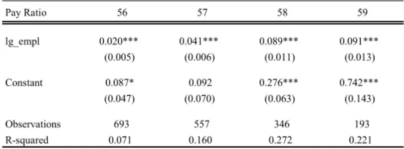
Table 4 shows the results. Although we run 36 individual regressions, the results are
surprisingly clear. Panel (A) includes all pay ratios in which hierarchy level 1 is compared
increases. As can be seen, the coefficient on firm size is initially insignificant (pay ratios
12, 13, 14, and 15). Beginning with pay ratio 16, it becomes positive and significant (pay
ratios 16, 17, 18, and 19). In addition, whenever the coefficient is significant, it is also
monotonically increasing in the pay ratio. For example, a one percent increase in firm
size increases the pay associated with hierarchy level 6 by 0.0375% relative to the pay
associated with hierarchy level 1. By comparison, the pay associated with hierarchy level
7 increases by 0.0883%, the pay associated with hierarchy level 8 increases by 0.162%,
and the pay associated with hierarchy level 9 increases by 0.179%–all relative to the pay
associated with hierarchy level 1. Thus, a one percent increase infirm size has a roughly
five times bigger impact on pay ratio 19 than it has on pay ratio 16.
Panels (B) to (D) include all pay ratios in which hierarchy levels 2, 3, or 4 are compared
to higher levels. The pattern is similar to that in Panel (A). Precisely, the coefficient on
firm size is initially insignificant–or, in one case (pay ratio 23), negative and significant–
and then positive and significant. Moreover, whenever the coefficient is significant, it is
also monotonically increasing in the pay ratio.12 Finally, Panels (E) to (H) include all pay
ratios in which hierarchy levels 5, 6, 7, or 8 are compared to higher levels. The pattern
is again similar, except that there is no region in which the coefficient on firm size is
insignificant. That is, the coefficient is always positive and significant, and it is always
monotonically increasing in the pay ratio.
Although we run 36 individual regressions, there appears to be a clear pattern in the
data. When lower hierarchy levels (1 to 5) are compared to one another, an increase in
firm size has no effect on within-firm pay inequality. In contrast, when higher hierarchy
levels (6 to 9) are compared to either one another or lower hierarchy levels, an increase
infirm size widens the pay gap between different hierarchy levels. The magnitude of this
effect increases with the distance between hierarchy levels. For instance, moving from
the 25th to the 75th percentile of the firm-size distribution–an increase in firm size of
1,565%–raises the pay associated with hierarchy level 9 by 280.1% relative to the pay
associated with hierarchy level 1. By comparison, the pay associated with hierarchy level
12There is one exception: in Panel (D), the coefficient on firm size decreases slightly when moving
6 increases only by 59.7% relative to the pay associated with hierarchy level 1.
Overall, we conclude that larger firms exhibit more pay inequality, as measured by
wage differentials between hierarchy levels (“pay ratios”). However, not all pay ratios
increase withfirm size, but only those involving hierarchy levels where managerial talent
is particularly important (levels 6 to 9). By contrast, pay ratios comparing lower hierarchy
levels to one another (levels 1 to 5) are invariant with respect tofirm size. Consequently,
an HR director’s pay (level 9) increases relative to the pay of an unskilled worker (level
1) asfirm size increases. However, the pay of an ordinary HR/Personnel officer (level 4)
does not increase relative to that of an unskilled worker.
Our results are not driven by industry composition effects. As is shown in Appendix
Table A3, all our results hold if we focus exclusively on within-industry variation. Our
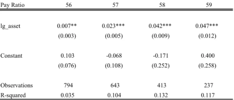
results are also similar if we measure firm size using eitherfirms’ sales or assets in lieu of
the number of employees (cf. Appendix Tables A1 and A2).
In Appendix Table A4, we show that our results are not driven by our choice of
winsorization. Rather than estimating 36 individual regressions–one for each pay ratio–
we lump all pay ratios together in a single regression and include pay ratio (i.e.,
hierarchy-level pair) fixed effects. Thus, the coefficient on firm size shows the average relation
between pay inequality and firm size within a given hierarchy-level pair. In our baseline
specification, we winsorize wages at 1% and firm size at 5%. In Panel (A), we continue to
winsorize wages at 1% but employ different winsorizations forfirm size. As is shown, our
results do not depend on how we winsorizefirm size. Similarly, in Panel (B), we continue
to winsorize firm size at 5% but employ different winsorizations for wages. As can be
seen, our results do not depend on how we winsorize wages. Finally, in Panel (C), we
winsorize both wages and firm size symmetrically at either 1%, 2.5%, 5%, or 10%. All
results are similar to those in Panels (A) and (B).
Appendix Table A4 shows the average relation between pay inequality and firm size
within a given hierarchy-level pair. In Appendix Table A5, we use quantile regressions
size affect different deciles of the pay-ratio distribution.13 We again include
hierarchy-level pair fixed effects. Hence, the coefficients are informative about how changes in
firm size affect the first, second, etc., decile of the pay-ratio distribution within a given
hierarchy-level pair. (Table 3 provides summary statistics showing quartiles of the
pay-ratio distribution separately for all 36 hierarchy-level pairs.) As can be seen, an increase
in firm size shifts the entire distribution of pay ratios upward, as evidenced by the fact
that all nine coefficients are positive and significant. However, the shift in the distribution
is not uniform: the coefficients are (almost monotonically) increasing across deciles, and
the coefficient associated with the ninth decile is more than three times larger than the
coefficient associated with thefirst decile. Thus, the relation between pay inequality and
firm size is mainly captured by the upper half of the pay-ratio distribution.
4.2
The Employer Size-Wage E
ff
ect Revisited
The invariance of “bottom-level” pay ratios–those comparing hierarchy levels 1 to 5
to one another–with regard to firm size raises questions. Are wages associated with
lower hierarchy levels individually invariant to firm size? Or do they merely increase (or
decrease) at a similar rate? To answer these questions, we shall now examine wagelevels
instead of ratios.
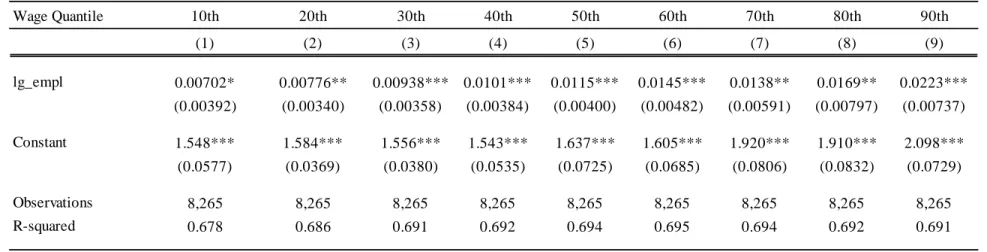
Table 5 presents the results. The first column, which combines all hierarchy levels,
includes hierarchy level fixed effects. Thus, the comparison is between small and large
firms within a given hierarchy level. As can be seen, the well documented employer
size-wage effect (e.g., Brown and Medoff (1989), Oi and Idson (1999)) also holds in our
data. Across all hierarchy levels, a one percent increase in firm size implies a wage
increase of 0.0126% on average. This magnitude is similar to the employer size-wage
effect documented in Brown and Medoff(1989, Table 1, 1b), who report a wage-firm size
elasticity of 0.013% using May CPS wage data.
But not all wages increase with firm size. Indeed, as the remaining columns show,
wages at lower hierarchy levels (1 to 5) do not increase with firm size–they are either
invariant to firm size or, if anything, slightly decreasing. In contrast, wages at higher
hierarchy levels (6 to 9) increase with firm size. For these wages, the rate of increase is
larger at higher hierarchy levels, which explains why “top-level” pay ratios, such as 78,
79, or 89, are all increasing infirm size.
Table 5 establishes two main results. First, while the employer size-wage effect also
holds in our data–wages are increasing withfirm size on average–it is entirely driven by
the upper tail of the wage distribution. Second, and equally important, the invariance of
“bottom-level” pay ratios with respect tofirm size is not driven by wages in the numerator
and denominator both increasing (or decreasing) at a similar rate. Rather, both wages
are individually invariant with respect to firm size.
4.3
Pay Inequality and Firm Growth
We already mentioned that our results hold if we focus exclusively on within-industry
variation (cf. Appendix Table A3). In what follows, we focus on within-firm variation,
thus accounting for any unobserved time-invariant heterogeneity acrossfirms.
Our ability to include firm fixed effects is limited by sample size considerations. As
mentioned earlier, IDS samples firms multiple times. The average sampling frequency
is 3.7 times, and the median is three times. However, not every sampling includes all
hierarchy levels within a given firm. As a consequence, some pay ratios have relatively
few within-firm repeat observations. Given this limitation, we form two broad groups of
pay ratios. One consists of “top-bottom” (e.g., 17, 18, 19, 27, 28, etc.) and “top-level”
(e.g., 67, 78, 89, etc.) pay ratios. These are the pay ratios that are significantly related
tofirm size in Table 4. The other group consists of “bottom-level” (e.g., 12, 23, 34, etc.)
pay ratios, i.e., pay ratios that compare lower hierarchy levels to one another. These pay
ratios arenot significantly related tofirm size in Table 4. Together, both groups span all
possible 36 pay ratios.
The question of interest is whether our main results continue to hold if we include
firm fixed effects. That is, does “top-bottom” and “top-level” pay inequality–but not
form broad groups of pay ratios, we can include hierarchy pair fixed effects and even
hierarchy pair × firm fixed effects. Thus, the coefficient on firm size provides us with
the average relation between changes in pay inequality and changes infirm size over time
within a given hierarchy pair and firm.
Table 6 reports the results. Columns (1), (3), and (5) show the results for
“bottom-level” pay ratios, while columns (2), (4), and (6) show the results for “top-bottom” and
“top-level” pay ratios. Columns (1) and (2) includefirmfixed effects, columns (3) and (4)
include hierarchy pair and firm fixed effects, and columns (5) and (6) include hierarchy
pair×firmfixed effects. As in Table 4, all regressions include yearfixed effects. As can be
seen, the coefficient onfirm size is insignificant for “bottom-level” pay ratios. By contrast,
it is significant for “top-bottom” and “top-level” pay ratios even after including hierarchy
pair ×firmfixed effects. Together, these results suggest that pay disparities between top
and bottom hierarchy levels–but also between different top hierarchy levels–become
larger as firms grow over time. Equally important, the results confirm that our main
results are not driven by unobserved time-invariant heterogeneity across firms.
5
Operating Performance and Firm Value
If pay inequality is primarily a reflection of managerial talent or incentive provision,
we would expect firms with more inequality to have better operating performance and
higher valuations. By contrast, if pay inequality is merely a reflection of managerial
rent extraction, we would expect firms with more inequality to have worse operating
performance and lower valuations.
Given our previous results showing that pay inequality is positively related to firm
size, we want to make sure that we are not simply picking up correlations between firm
size and operating performance or firm value. For this reason, we run all regressions
both with and without firm-size controls. To see what this means conceptually, consider
the talent assignment hypothesis. If firm size was a perfect proxy for managerial talent,
we should see no variation in pay inequality among firms of similar size. However, firm
proxy for talent–consistent with our results in Section 4–but an imperfect one, and so
firms of the same size may hire managers of different talent.14 Those hiring more talented managers exhibit greater pay inequality. Thus, pay inequality may proxy for talent even
after controlling for firm size.15 In the data, there is much variation in pay inequality
among firms of similar size, consistent with the above argument.
To obtain a measure of pay inequality at the firm level, we compute for eachfirm-pay
ratio-year observation its percentile rank within the pay-ratio sample distribution in the
same year. (For example, pay ratio 19 at firm X in year Y lies at the Zth percentile
across all observations associated with pay ratio 19 in that year.) We then aggregate this
information at the firm level by computing the average percentile rank for each firm in
a given year.16 Lower average percentile ranks mean lower pay inequality. We lag our
measure of pay inequality by one year in all regressions.
Panel (A) of Table 7 examines the relation between within-firm pay inequality and
the firm’s return on assets (ROA). Column (1) shows that this relation is positive and
significant. In column (2), we control for firm size. As can be seen, the point estimate
is slightly smaller, and the result is statistically weaker. In columns (3) and 4), we use
industry-adjusted ROA as our dependent variable. Industry adjustments are done by
subtracting the industry median across all firms in Amadeus in the same 3-digit SIC
industry and year. As is shown, the results largely mirror those in columns (1) and
(2): there is a positive and significant relation between pay inequality and ROA, while
controlling for firm size lowers the point estimates and raises the standard errors.17
14A manager’s marginal product may be increasing in several factors, firm size being (only) one of
them. For instance, in Edmans and Gabaix (2011), managerial talent is assigned based on firm size as well asfirm risk. Similarly, in Eisfeldt and Kuhnen (2013),firms and managers form matches based on multiple characteristics.
15Even iffirm size was a perfect proxy for managerial talent, we would see variation in pay inequality
among firms of similar size if somefirms were acting suboptimally, paying either too much or too little relative to what is optimal. We thank an anonymous referee for pointing this out.
16Assigning equal weight to all 36 pay ratios may lead to situations in whichfirms with large
“top-bottom” pay ratios (e.g., 18, 29)–high-inequalityfirms by any sensible standards–are (mis-)classified as low-inequalityfirms only because they have compressed “mid-level” (e.g., 34, 45) or “bottom-level” (e.g., 12, 23) pay ratios. For this reason, we only use “top-bottom” pay ratios when computing our firm-level measure of pay inequality.
Panel (B) considers the relation between pay inequality and firm value (Tobin’s Q).
Tobin’s Q is the market value of assets divided by the book value of assets, where the
market value of assets is the book value of assets plus the market value of common
stock minus the sum of the book value of common stock and balance sheet deferred
taxes. Given that Amadeus does not provide estimates of market values, we must limit
ourselves to publicly traded firms in the UK and construct measures of firm value using
Datastream. The results largely mirror those in Panel (A). In particular, there is a positive
and significant association between pay inequality andfirm value, which holds even after
controlling for firm size and industry-adjusting Tobin’s Q.
In sum, the results in Table 7 suggest that high pay-inequality firms are not worse
performers. On the contrary, they appear to have better operating performance and
higher Tobin’s Q.
6
Competition and Governance
The results in Section 5 are inconsistent with managerial rent extraction. By contrast,
all the results so far are consistent with both talent assignment and incentive provision.
In principle, both hypotheses could be in operation, given that they are not mutually
exclusive. In the following, we present additional evidence trying to distinguish between
the two hypotheses. The underlying idea is that if moral hazard is the key channel, we
should see stronger results in environments where moral hazard is potentially more severe,
e.g., in less competitive industries (Giroud and Mueller (2010, 2011)) or among firms
with weaker governance. On the other hand, if talent assignment is the key channel, our
results should be stronger inmore competitive industries, since there is more competition
for managerial talent. If better governance results in a better assignment of managerial
talent, our results should also be stronger among better governed firms.18
Table 8 examines whether our results are stronger in less or more competitive
in-dustries, or among firms with weaker or better governance. Our measures of industry
concentration are the Herfindahl-Hirschmann Index (HHI), the Lerner Index, and the
Top 5 concentration ratio. The HHI is defined as the sum of squared market shares in
a given industry and year. Industries are based on 3-digit SIC codes. Market shares are
based on firms’ sales using all firms in Amadeus. The Lerner Index is computed as in
Aghion et al. (2005). It is the average price-cost margin across allfirms in Amadeus in a
given 3-digit SIC industry and year. At thefirm-year level, the price-cost margin is
com-puted as operating profits minus depreciation, provisions, and financial costs divided by
sales. The Top 5 concentration ratio is the sum of market shares of the largest fivefirms
in a given 3-digit SIC industry and year. Market shares are based on firms’ sales using
allfirms in Amadeus. Our measures of firm-level governance are board independence and
blockholder ownership. Board independence is the ratio of the number of independent
directors to total board size using data from BoardEx UK. Blockholder ownership is total
direct ownership by all blockholders of a firm with an ownership stake of 5% or more
using data from the Osiris database.
In Panels (A) to (C), we examine whether our results are stronger in less or more
competitive industries. Sample splits are based on industry medians, i.e., “low” refers to
industries with below-median values of the HHI, Lerner Index, and Top 5 concentration
ratio, respectively (“competitive industries”). Columns (1) to (4) consider the relation
between pay inequality and the firm’s return on assets (ROA) based on the empirical
specification used in Table 7. Columns (5) and (6) consider the relation between pay
inequality and firm size based on the empirical specification used in Table 6. In Panel
(A), industry concentration is measured using the HHI. As is shown, our results are much
stronger in competitive industries. Indeed, the coefficients are only significant in those
industries. That being said, the coefficients in competitive and concentrated industries
are not always significantly different from each other. While the difference is significant
in the ROA regressions (p-values of 0.031 and 0.037, respectively), it is not significant in
thefirm-size regressions (p-value of 0.156). A similar picture emerges in Panel (B), where
industry concentration is measured using the Lerner Index, and in Panel (C), where it is
measured using the Top 5 concentration ratio.
In Panels (D) and (E), we examine whether our results are stronger among firms with
blockholder ownership, wefind that our results are stronger among better governedfirms.
Similar to above, however, the coefficients associated with weak- and strong-governance
firms may not be significantly different from each other.
Overall, the results in Table 8 provide support for the talent assignment hypothesis.
Using different measures of industry concentration andfirm-level governance, wefind that
our results are stronger in more competitive industries and among better governedfirms,
albeit the differences between low- and high-competition industries, or between weak- and
strong-governance firms, are not always significant.
7
Is Pay Inequality Priced by the Market?
This section examines if within-firm pay inequality is priced by the market. To study
the relation between pay inequality and equity returns, we form a hedge portfolio that is
long in high-inequality firms and short in low-inequality firms. Our stock price data are
from Datastream. Our measure of pay inequality is the same as in Section 5. To reflect
changes in pay inequality over time, we rebalance portfolios at the beginning of each
year. We compute both equal- and value-weighted portfolio returns. Portfolio weights are
constructed using firms’ end-of-year market capitalizations. A firm is classified as “high
inequality” in year if its pay inequality measure in year−1lies in the top tercile across all firms in our sample. Similarly, a firm is classified as “low inequality” in year if its
pay inequality measure in year −1 lies in the bottom tercile of the sample distribution.
The sample period is from 1/2006 to 9/2014 (105 months). Excess returns are computed
by subtracting 3-month UK Treasury bill returns from raw returns.
Table 9 reports results from time-series regressions of monthly excess returns. For
brevity, the table only displays the intercept, or alpha (), of each regression. Panel
(A) shows results for the inequality hedge portfolio. Panels (B) and (C) show results
separately for the high- and low-inequality portfolio. In all three panels, columns (1)
and (2) show results for value-weighted portfolios, while columns (3) and (4) show results
Finance and Investment at the University of Exeter.19
Columns (1) and (3) show results from regressions of monthly excess returns on an
intercept and the market factor (RMRF). As can be seen, the alpha associated with the
inequality hedge portfolio is positive and significant. In both value- and equal-weighted
regressions, the alpha associated with the high-inequality portfolio is positive, while the
alpha associated with the low-inequality portfolio is negative. Notably, the alpha
as-sociated with the high-inequality portfolio is small relative to that asas-sociated with the
low-inequality portfolio. Hence, most of the abnormal return associated with the hedge
portfolio is driven by the low-inequality portfolio. Columns (2) and (4) show results from
estimating the Carhart (1997) four-factor model, which includes, besides the intercept
and RMRF, the book-to-market factor (HML), size factor (SMB), and momentum factor
(UMD). The results mirror those obtained from using the market model. In both
value-and equal-weighted regressions, the alpha associated with the inequality hedge portfolio
is positive and significant. And again, most of the abnormal return associated with the
hedge portfolio is driven by the low-inequality portfolio.
What accounts for the positive alpha associated with the inequality hedge portfolio?
One interpretation, which is consistent with our previous results, is that high-inequality
firms attract better managerial talent, and this is not fully captured by the market.
This interpretation is consistent with Edmans (2011), who finds that the market does
not fully capture intangibles (specifically, employee satisfaction). In our case, the scope
for mispricing is especially large, since our within-firm pay-level data are not publicly
available. Alternatively, there is the possibility that pay inequality may be correlated
with firm characteristics that have been shown to affect stock returns. To explore this
possibility, we now turn to Fama-MacBeth regressions, allowing us to include a wide array
of control variables.
Table 10 reports Fama-MacBeth coefficients from monthly cross-sectional regressions
of individual stock returns on a “high inequality” dummy and control variables. The
dummy is equal to one if a firm’s pay inequality measure in year −1 lies in the top
tercile of the sample distribution and zero if it lies in the bottom tercile. The sample is
restricted to firms in the top and bottom terciles. Our measure of pay inequality is the
same as in Table 9. Hence, firms classified as “high inequality” are the same firms that
make up the high-inequality portfolio in our time-series regressions. Control variables
include size (market equity), book-to-market, dividend yield, trading volume, and stock
price, all lagged, as well as compound returns from months -3 to -2 (Ret2-3), -6 to
-4 (Ret4-6), and -12 to -7 (Ret7-12). These controls are standard in Fama-MacBeth
regressions of this sort (e.g., Brennan, Chordia, and Subrahmanyam (1998), Gompers,
Ishii, and Metrick (2003), Giroud and Mueller (2011), Edmans (2011)).
The results in Table 10 broadly confirm those in Table 9. As Gompers, Ishii, and
Metrick (2003) point out, the dummy coefficient in the Fama-MacBeth regression can be
interpreted as an abnormal return. In column (1), which does not include any controls,
the abnormal return is similar to what we found previously in Table 9. In column (2),
which includes size and book-to-market as controls, the abnormal return in slightly lower.
Lastly, in column (3), which includes the full set of controls, the abnormal return to
high-inequalityfirms (relative to low-inequalityfirms) is 0.954% and significant at the 5% level.
Thus, we may conclude that the explanatory power of pay inequality for equity returns
does not simply arise because pay inequality is correlated with firm characteristics that
have been shown to be correlated with returns.
8
Earnings Surprises
Our results in Section 7 are consistent with the view that high-inequality firms attract
better managerial talent, and this is not fully captured by the market. To provide further
evidence on mispricing, we now study earnings surprises. Under a mispricing channel,
investors do not fully anticipate the earnings by high-inequalityfirms. That is, investors
are (positively) surprised.
Following Core, Guay, and Rusticus (2006), Giroud and Mueller (2011), and Edmans
(2011), we use analysts’ earnings forecasts to proxy for investors’ expectations. Data on
(I/B/E/S). Analysts’ forecast error (or “earnings surprise”) is the firm’s actual earnings
per share at thefiscal year-end minus the (mean or median) I/B/E/S consensus forecast
of earnings per share, scaled down by the firm’s stock price two months prior. We use
the I/B/E/S consensus forecast eight months before the fiscal year-end to ensure that
analysts know the previous year’s earnings when making their forecasts. To mitigate the
effect of outliers, we drop observations for which the forecast error is larger than 10% of
the stock price in the month of the forecast (e.g., Lim (2001), Teoh and Wong (2002)).
Finally, we require that a company be followed by at least five analysts to ensure that
consensus forecasts constitute reliable proxies of market expectations (e.g., Easterwood
and Nutt (1999), Loha and Mianc (2006)).
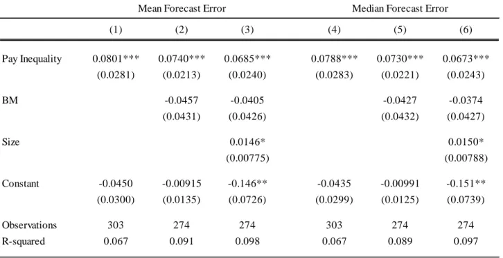
Table 11 presents the results. Columns (1) to (3) consider analysts’ forecast errors
based on mean I/B/E/S consensus forecasts, while columns (4) to (6) consider analysts’
forecast errors based on median I/B/E/S consensus forecasts. Pay inequality is the same
(lagged) measure as in Section 5, where we studied the relation between pay inequality
and firms’ earnings. Control variables include size (market equity) and book-to-market.
As can be seen, regardless of which controls we include, and regardless of whether we
consider mean or median I/B/E/S consensus forecasts, firms with higher pay inequality
exhibit significantly larger earnings surprises. Thus, the market is indeed surprised by
the earnings of high-inequality firms, consistent with a mispricing channel.
9
Concluding Remarks
Using a proprietary data set of public and private firms in the UK, we study how
within-firm pay inequality varies acrossfirms, how it relates tofirms’ operating performance and
valuations, and whether it is priced by the market. Wefind that high-inequalityfirms are
larger, consistent with theories emphasizing the efficient assignment of managerial talent.
In addition, we find that high-inequality firms have higher valuations, better operating
performance, and higher equity returns. The latter result suggests that managerial talent
is not fully priced by the market, consistent with our findings that high-inequality firms
Aggregate income inequality has risen steadily over the past decades.20 While this is
arguably speculative, our results suggest that some of this rise may be related to firm
growth.21 Between 1986 and 2010, average employment by the 50 (100) largest firms
in the U.S. has risen by 55.8% (53.0%). Likewise, over the same time period, average
employment by the 50 (100) largest firms in the UK has risen by 51.3% (43.5%). In
untabulated results, we explore the relation betweenfirm growth by the largestfirms in a
country and aggregate income inequality, as measured by the log 90/10 wage differential,
based on a sample of 16 developed countries. Irrespective of whether we consider the 50
or 100 largest firms in a country, we find a positive and significant association between
firm growth and aggregate income inequality at the country level. Thus, part of what
may be perceived as a global trend toward more wage inequality may be driven by an
increase in employment by the largestfirms in the economy.
10
References
Aghion, Philippe, Nick Bloom, Richard Blundell, Rachel Griffith, and Peter Howitt,
2005, Competition and Innovation: An Inverted-U Relationship, Quarterly Journal
of Economics 120, 701-728.
Alesina, Alberto, and Dani Rodrik, 1994, Distributive Politics and Economic Growth,
Quarterly Journal of Economics 109, 465-490.
Alvarez, Jorge, Niklas Engbom, and Christian Moser, 2015, Firms and the Decline of
Earnings Inequality in Brazil, mimeo, Princeton University.
Atkinson, Anthony, Thomas Piketty, and Emmanuel Saez, 2011, Top Incomes in the
Long Run of History, Journal of Economic Literature 49, 3-71.
Barth, Erling, Alex Bryson, James Davis, and Richard Freeman, 2016, It’s Where You
20See Atkinson, Piketty, and Saez (2011) for a review of the literature.
21Section 4.1 shows that largerfirms exhibit more within-firm pay inequality. Section 4.3 shows that
Work: Increases in the Dispersion of Earnings across Establishments and Individuals
in the United States, Journal of Labor Economics 34, S67-S97.
Bebchuk, Lucian, and Jesse Fried, 2004, Pay Without Performance: The Unfulfilled
Promise of Executive Compensation. Cambridge, MA: Harvard University Press.
Bebchuk, Lucian, Martijn Cremers, and Urs Peyer, 2011, The CEO Pay Slice, Journal
of Financial Economics 102, 199-221.
Bertrand, Marianne, and Sendhil Mullainathan, 1999, Is There Discretion in Wage
Set-ting? A Test Using Takeover Legislation, Rand Journal of Economics 30, 535—554.
Bertrand, Marianne, and Sendhil Mullainathan, 2003, Enjoying the Quiet Life?
Cor-porate Governance and Managerial Preferences, Journal of Political Economy 111,
1043-1075.
Breza, Emily, Supreet Kaur, and Yogita Shamdasani, 2016, The Morale Effects of Pay
Inequality, NBER Working Paper 22491.
Brown, Charles, and James Medoff, 1989, The Employer Size-Wage Effect, Journal of
Political Economy 97, 1027-1059.
Card, David, Jörg Heining, and Patrick Kline, 2013, Workplace Heterogeneity and the
Rise of West German Wage Inequality, Quarterly Journal of Economics 128,
967-1015.
Carhart, Mark, 1997, On Persistence in Mutual Fund Performance, Journal of Finance
52, 57-82.
Corak, Miles, 2013, Income Inequality, Equality of Opportunity, and Intergenerational
Mobility, Journal of Economic Perspectives 27, 79-102.
Core, John, Wayne Guay, and Tjomme Rusticus, 2006, Does Weak Governance Cause
Weak Stock Returns? An Examination of Firm Operating Performance and
Cronqvist, Henrik, Fredrik Heyman, Mattias Nilsson, Helena Svaleryd, and Jonas
Vla-chos, 2009, Do Entrenched Managers Pay Their Workers More? Journal of Finance
64, 309-339.
Easterly, William, 2007, Inequality Does Cause Underdevelopment: Insights from a New
Instrument, Journal of Development Economics 84, 755-776.
Easterwood, John, and Stacey Nutt, 1999, Inefficiency in Analysts’ Earnings Forecasts:
Systematic Misreaction or Systematic Optimism? Journal of Finance 54, 1777-1797.
Edmans, Alex, 2011, Does the Stock Market Fully Value Intangibles? Employee
Satis-faction and Equity Prices, Journal of Financial Economics 101, 621-640.
Edmans, Alex, and Xavier Gabaix, 2011, The Effect of Risk on the CEO Market, Review
of Financial Studies 24, 2822-2863.
Edmans, Alex, and Xavier Gabaix, 2016, Executive Compensation: A Modern Primer,
Journal of Economic Literature, forthcoming.
Edmans, Alex, Xavier Gabaix, and Augustin Landier, 2009, A Multiplicative Model of
Optimal CEO Incentives in Market Equilibrium, Review of Financial Studies 22,
4881-4917.
Edmans, Alex, Itay Goldstein, and John Zhu, 2013, Contracting with Synergies, mimeo,
London Business School.
Eisfeldt, Andrea, and Camelia Kuhnen, 2013, CEO Turnover in a Competitive
Assign-ment Framework, Journal of Financial Economics 109, 351-372.
Frydman, Carola, and Dirk Jenter, 2010, CEO Compensation, Annual Review of
Finan-cial Economics 2, 75-102.
Gabaix, Xavier, and Augustin Landier, 2008, Why Has CEO Pay Increased So Much?
Gabaix, Xavier, Augustin Landier, and Julien Sauvagnat, 2014, CEO Pay and Firm Size:
An Update After the Crisis, Economic Journal 124, F40-F59.
Gayle, George-Levi, and Robert Miller, 2009, Has Moral Hazard Become a More
Impor-tant Factor in Managerial Compensation? American Economic Review 99,
1740-1769.
Giroud, Xavier, and Holger Mueller, 2010, Does Corporate Governance Matter in
Com-petitive Industries? Journal of Financial Economics 95, 312-331.
Giroud, Xavier, and Holger Mueller, 2011, Corporate Governance, Product Market
Com-petition, and Equity Prices, Journal of Finance 66, 563-600.
Gompers, Paul, Joy Ishii, and Andrew Metrick, 2003, Corporate Governance and Equity
Prices, Quarterly Journal of Economics 118, 107-155.
Gregory, Alan, Rajesh Tharyan, and Angela Christidis, 2013, Constructing and Testing
Alternative Versions of the Fama-French and Carhart Models in the UK, Journal of
Business Finance and Accounting 40, 172-214.
Groen-Xu, Moqi, Peggy Huang, and Yiqing Lu, 2016, Subjective Performance Reviews
and Stock Returns, mimeo, London School of Economics.
International Monetary Fund, 2014, Redistribution, Inequality, and Growth, IMF Staff
Discussion Note.
Kaplan, Steven, and Joshua Rauh, 2010, Wall Street and Main Street: What Contributes
to the Rise in the Highest Incomes? Review of Financial Studies 23, 1004-1050.
Kaplan, Steven, and Joshua Rauh, 2013, It’s the Market: The Broad-Based Rise in the
Return to Top Talent, Journal of Economic Perspectives 27, 35-56.
Koenker, Roger, and Gilbert Basset, 1978, Regression Quantiles, Econometrica 46, 33-51.
Koenker, Roger, and Kevin Hallock, 2001, Quantile Regression, Journal of Economic