Index Catalog // Carolina Digital Repository

(1)

Vertical Integration of Multiple High-Dimensional

Datasets

Eric F. Lock

A dissertation submitted to the faculty of the University of North Carolina at Chapel Hill in partial fulfillment of the requirements for the degree of Doctor of Philosophy in the Department of Statistics and Operations Research.

Chapel Hill 2012

Approved by:

(2)

c 2012 Eric F. Lock

(3)

Abstract

ERIC F. LOCK: Vertical Integration of Multiple High-Dimensional Datasets.

(Under the direction of Andrew B. Nobel and J. S. Marron.)

Research in genomics and related fields now often requires the analysis ofmulti-block

data, in which multiple high-dimensional types of data are available for a common set of objects. We introduce Joint and Individual Variation Explained (JIVE), a general decomposition of variation for the integrated analysis of multi-block datasets. The de-composition consists of three terms: a low-rank approximation capturing joint variation across datatypes, low-rank approximations for structured variation individual to each datatype, and residual noise. JIVE quantifies the amount of joint variation between datatypes, reduces the dimensionality of the data, and allows for the visual explo-ration of joint and individual structure. JIVE is an extension of Principal Components Analysis and has clear advantages over popular two-block methods such as Canonical Correlation and Partial Least Squares.

Research in a number of fields also requires the analysis of multi-way data. Multi-way data take the form of a three (or higher) dimensional array. We compare several existing factorization methods for multi-way data, and we show that these methods belong to the same unified framework.

The final portion of this dissertation concerns biclustering. We introduce an ap-proach to biclustering a binary data matrix, and discuss the application of biclustering to classification problems.

(4)

Acknowledgments

Much of the work described in this dissertation is collaborative, and I am very grateful for all of the help I have received. In particular, I would like to thank:

• My advisors Andrew Nobel and Steve Marron, for their patience, dedication, and many insightful comments.

• My committee members Haipeng Shen, Wei Sun and Ivan Rusyn, for their helpful criticism and suggestions.

• Ivan Rusyn, Katherine Hoadley, and Blair Bradford for providing data and pa-tiently explaining scientific questions and concepts.

• Andrey Shabalin, Gen Li, Fred Wright, Phil Howard and many others for their additional helpful comments.

(5)

List of Figures

2.1 PCA plot of gene expression data for 134 mice, colored by genetic strain with ‘+’ for alcohol treated and ‘O’ for control samples. The diagonal panels give one-dimensional projections on the first three principal components; the off-diagonal panels give scatterplots for each pair of principal components. The black curve shown on each diagonal panel gives a kernel density estimate for the overall distri-bution of the principal component scores, and the colored curves give kernal density estimates within each strain. In this PCA view we see that the first two components distinguish certain strains, while

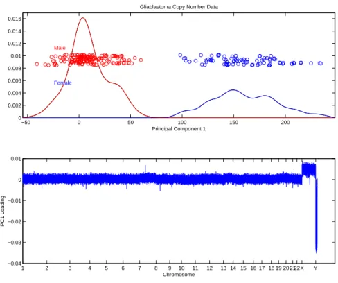
the third distinguishes the treated samples from the controls. . . 20 2.2 Projections on the first principal component for gliablastoma copy

number data (top), and the loading vector ordered by genomic lo-cation (bottom). The first principal component distinguishes male and female, and the loadings indicate involvement of chromosomes

X and Y. . . 21

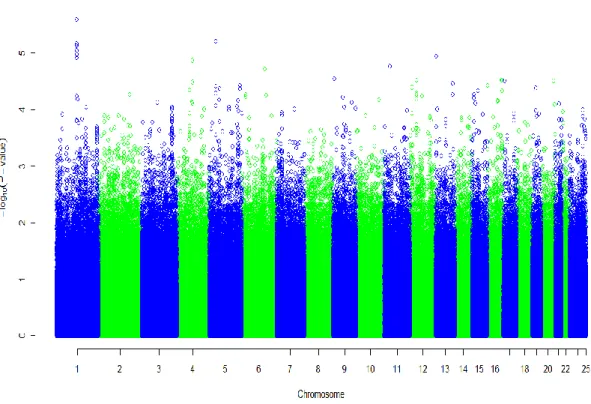
3.1 GWAS measures the strength of association between SNPs and the first principal component of toxicity on 81 cell lines. The SNPs are ordered by chromosomal location on the horizontal axis, and −log₁₀(P-value) for the signficance of the association between each

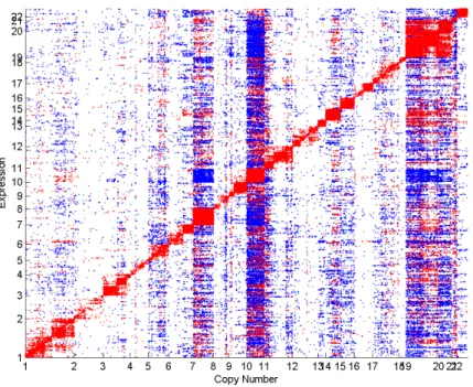
SNP and the first principal component is shown. . . 26 3.2 Plot of significant correlations between copy number and gene

ex-pression data on 234 GBM tumor samples. Both copy number (hor-izontal axis) and gene expression (vertical axis) are ordered by ge-nomic location. Points are colored red (blue) if the correlation be-tween the corresponding gene - copy number pair is significant and

positive (negative). . . 27 3.3 PLS plots for gene expression and metabolomic data on 134 mice,

colored by genetic strain with ’+’ for alcohol treated and ’O’ for control samples. Scatterplots of the first 2 pairs of PLS directions

(expression vs metabolite scores) are shown. . . 31

(10)

4.1 Depiction of the JIVE decomposition for two datasets. The data are approximated by a low rank matrix of joint variation and low rank

matrices giving structured variation unique to X1 and X2. . . 37

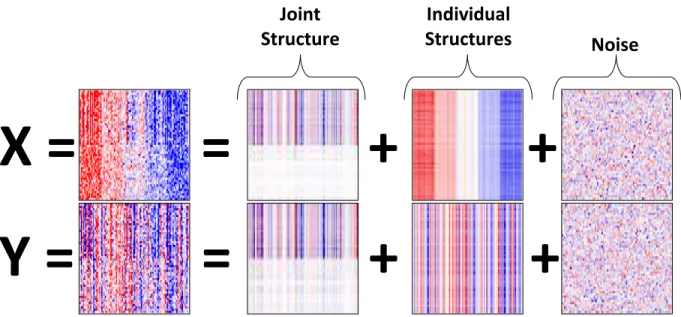
4.2 X and Y are generated by adding together joint structure, individ-ual structure, and noise. Blue corresponds to negative values, red

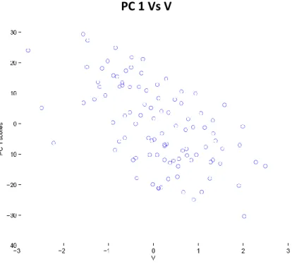
positive values. . . 47 4.3 Scatterplot of the first consensus principal component scores Vs the

joint signal V. The scores are weakly associated with the joint signal. . 48 4.4 The first pair of PLS, and CCA, directions for Xand Y. Panels (A)

and (B) show a weak association between the PLS scores and the joint signal V. Points are colored by simulated class in both X and

Y, and are more highly associated with V within each class. The first pair of CCA directions correlate with each other (F), but not the common signal V (D and E). This illustrates the tendency of

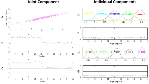
CCA to overfit. . . 49 4.5 Scores and loadings for joint and individual components in the JIVE

decomposition. Joint scores are highly associated with the common signal V (panel A). Individual scores distinguish classes specific to

X and Y (D and F). Joint loadings (B and C) show a strong effect (difference from zero) on half of the variables inX andY. Individual

loadings (E and G) show a similar effect on all variables in X and Y. . 50 4.6 JIVE estimates for joint structure, individual structure, and noise.

Blue corresponds to negative values, red positive values. . . 51 4.7 Simulation based on miRNA, GE and CN data. Columns are

per-muted within each datatype so that samples are not associated. A

common signal is then added to 5% of the rows in each datatypes. . . 52 4.8 Scores for the first Consensus PC of the concatenated data, colored

by cluster. Kernel density curves are shown for all scores (black) and the two clusters (red and blue). The two clusters (representing

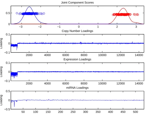
common signal) are not well distinguished. . . 52 4.9 Joint component scores and loadings. Scores are colored by

artifi-cial cluster and show good separability. Loadings for CN, GE, and miRNA are ordered so that the first 5% have joint signal added, and

(11)

4.10 Sum of squared residuals in the simulated model (green), the fitted model with true ranks (blue) and the fitted model under permuta-tion testing (red) in 100 randomly generated simulapermuta-tions, ordered

by the amount of simulated error. . . 55 4.11 JIVE estimates for joint structure and individual structure on the

GBM data. Blue corresponds to negative values, red positive values. . . 58 4.12 Percentage of variation (sum of squares) explained by estimated

joint structure, individual structure and residual noise for miRNA

and gene expression data. . . 59 4.13 Heatmaps of low-rank estimations for joint structure, individual

structurem and residual noise in the gene expression (top) and miRNA (bottom) data. Blue corresponds to negative values, Red positive

values. . . 60 4.14 Scatterplots of sample scores for the first two joint components,

first two individual miRNA components, and first two individual gene expression components. Samples are colored by subtype: Mes-enchymal (yellow), Proneural (blue), Neural (green) and Classical (red). Samples colored black were assayed after the initial subtype

analysis, and are considered unclassified. . . 61 4.15 Plot of gene-miRNA correlations (A), and scores and loadings for the

first two sparse joint components (B-E). In (A), gene-miRNA pairs are colored red if they have a significant positive correlation and blue if they have a significant negative correlation (P < 10−5_{). Panels}

(B) and (D) show sample scores for the first two joint components, colored by subtype. Panels (C) and (E) display gene-miRNA pairs where each have non-zero loadings. Pairs are colored red if both gene and miRNA loadings have the same sign, blue otherwise. In panels (A), (C) and (E) genes and miRNAs are ordered separately

by average linkage correlation clustering. . . 63

(12)

4.16 Network of predicted gene-miRNA interactions for the first two sparse joint components. Gene-miRNA pairs are linked if the miRNA is predicted to target the gene in two or more of the four databases

miRanda, Pictar, RNA22 and TargetScan. Genes are shown as

cir-cles, and miRNAs are shown as squares. All predicted targets are shown between the 10 miRNAs with the largest absolute loading and the 10 genes with the largest absolute loading, for both com-ponents. Genes and miRNAs with a positive loading are colored red, and with a negative loading are colored blue. The icon size is

proportional to the absolute loading. . . 64 4.17 Horizontal JIVE decomposition on two sample sets. Low-rank

ap-proximations are given for joint structure and individual structure

within each sample set. . . 66 4.18 Heatmaps of low-rank estimations for joint structure and individual

structure in the Basal (left) and Luminal (right) samples. Blue

corresponds to negative values, Red positive values. . . 68 4.19 Heatmaps of low-rank estimates for individual structure in the

Lu-minal and Basal samples. The genes are ordered separately in each

dataset. Blue corresponds to negative values, Red positive values. . . . 68 4.20 Scatterplots of sample projections on the first two joint components,

first two individual components from the Basal samples, and first two individual components from the Luminal samples. Basal sam-ples are colored red, Luminal A samsam-ples are colored blue, and

Lu-minal B samples are colored cyan. . . 69 4.21 Illustration of simulated data. We add signal such that some

sam-ples in each class are distinguished on both X1 and X2, some are

distinguished on X1 only and some are distinguished on X2 only. . . 73

4.22 JIVE component scores for joint and indivual structure, colored by simulated class (1 or -1). Samples that were truly distinguished on both datasets are marked ’O’, samples distinguish on only X1 are

marked ’+’, samples distinguished on only X2 are marked ’3’. . . 74

4.23 JIVE component scores for joint and indivual structure after re-moving variables not associated with the outcome, colored by simu-lated class (1 or -1). Samples that were truly distinguished on both datasets are marked ’O’, samples distinguish on onlyX1 are marked

(13)

4.24 Percentage of variation (sum of squares) explained by estimated joint structure, individual structure and residual noise for copy num-ber and DNA methylation. Panel A dispays the results for the full JIVE analysis, panel B displays the results for the supervised JIVE

analysis. . . 76 4.25 Scatterplots of sample projections on the first two joint components,

first two individual copy number components, and first two individ-ual methylation components. Results for the full JIVE analysis are shown in poanel A, and results for the supervised JIVE analysis are shown in panel B. Basal samples are colored red, Luminal A sam-ples are colored blue, and Luminal B samsam-ples are colored cyan, Her2

samples are colored yellow, and Normal samples are colored green. . . 77 4.26 Illustration of the factorial JIVE model for three datatypes. Low

rank approximations are used for all three datatypes (black); for X1

and X2 (purple), X1 andX3 (turquoise), X2 and X3 (yellow-green);

and each of X1 (blue),X2 (red) and X3 (green) individually. . . 83

5.1 Application of PVD, Tucker, Parafac and SVD factorizations to facial image data. Panel A displays the sum of squared residu-als versus the degrees of freedom used to fit the model for each method. Panel B displays three facial images (at left), and their reconstructions using the four methods. Each reconstruction uses similar degrees of freedom, close to the vertical line in panel A. The Parafac approximation shown uses 72,480 (r = 120) degrees of freedom, PVD uses 70,252 (A = B = 13), Tucker uses 73,001

(r1 =r2 =r3 = 37), and SVD uses 74,928 (r = 7). . . 95

6.1 Illustration of several biclusters (colored) within a data matrix. Note that biclusters may overlap, and are not necessarily on a contiguous

set of rows or columns. . . 97 6.2 A heatmap of all gene expression data for 137 mouse samples, with

a positive (red) and negative (green) bicluster identified by LAS. Columns correspond to mice and rows correspond to genes; red

val-ues are high and green are low. . . 99

(14)

6.3 A heatmap of the genes identified to have a significant bicluster on TCE mouse samples with no significant counterpart on control sam-ples is shown on the left, and the columns selected for each bicluster are shown on the right. Red corresponds to high expression, and green low expression. The TCE colums selected have visisbly higher

(15)

List of Tables

1.1 Examples with multiple high-dimensional datatypes. . . 3 1.2 Examples of multi-way data arrays. . . 4

4.1 SWISS scores for TCGA subtypes. Lower scores indicate more

sub-type distinction. . . 62

5.1 Data examples where the objects are matrices of the same dimension. . 84

(16)

Chapter 1 Introduction

1.1 Motivation

The field of exploratory data analysis encompasses a wide range of statistical methods that are used to identify, summarize and display the main characteristics of a dataset. Exploratory methods are not meant to answer pre-defined questions (this is sometimes calledconfirmatory analysis). Rather, they are meant to aid our understanding of “the big picture” in a dataset. John Tukey summarizes the need for exploratory analysis with the quote below.

[Science] does not begin with a tidy question. Nor does it end with a tidy answer. [...] We need to think about science and engineering more broadly than the narrow, inadequate paradigm of a straight line from question to answer. (Tukey, 1980)

(17)

scatterplot). However, technological and computational advances are producing com-plex datasets that do not fit this simple paradigm and require the development of new exploratory techniques.

One kind of data that does not fit the standard paradigm is high-dimensional data, in which a large number of variables are measured for each object. Many fields of research now involve the analysis of high-dimensional data. Text mining, image anal-ysis, e-commerce and computational biology, for example, all involve datatypes where hundreds or thousands of variables (e.g., word frequencies, pixel intensities, customer browsing history, and molecule concentrations) are measured for each object of interest (e.g., documents, images, customers, and tissue samples). Often, the number of vari-ables exceeds the number of available objects, resulting in High Dimension Low Sample Size (HDLSS) data. Standard exploratory approaches that study the distribution of each variable and relationships between variable pairs suffer from “information over-load” on high-dimensional data. Furthermore, classical statistical methods typically assume the sample size is significantly larger than the number of variables. Hence, interest in and statistical research on high-dimensional and HDLSS data has grown rapidly in recent years.

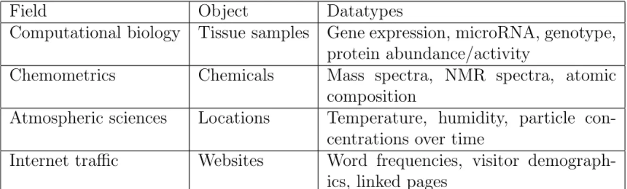
A more complex kind of dataset is one in which multiple large and fundamentally different sets of variables are available for a common set of objects. This is an in-creasingly common scenario in several fields of research that involve the collection of multiple types of high-dimensional data. Table 1.1 gives very diverse examples of such data objects. We refer to data of this structure as multi-block data.

Multi-block data are especially common in biomedical studies, where a number of technologies are now commonly used to collect diverse kinds of information on the same set of organisms or tissue samples. The amount of available biological data from multiple platforms and technologies is expanding rapidly. The 2011 Online Database

(18)

Field Object Datatypes

Computational biology Tissue samples Gene expression, microRNA, genotype, protein abundance/activity

Chemometrics Chemicals Mass spectra, NMR spectra, atomic composition

Atmospheric sciences Locations Temperature, humidity, particle con-centrations over time

Internet traffic Websites Word frequencies, visitor demograph-ics, linked pages

Table 1.1: Examples with multiple high-dimensional datatypes.

collection ofNucleic Acids Research lists 1330 publicly available databases that measure different aspects of molecular and cell biology (Galberin and Cochrane, 2011). Large online databases such as ArrayExpress (Parkinson et al., 2009) and the UCSC Genome-browser (Rhead et al., 2010) often contain multiple disparate datatypes collected from a common set of samples. Large-scale projects like The Human Connectome Project (Sporns, Tononi and Kotter, 2005) and The Cancer Genome Atlas (TCGA Research Network, 2008) focus on the integrated analysis of multiple datatypes.

Well established multivariate methods can be used to separately analyze different datatypes measured on the same set of objects. However, individual analysis of each datatype will not capture the critical associations and potential causal relationships between datatypes. Furthermore, each datatype can impart unique and useful infor-mation. There is a strong need for new statistical methods that explore associations between multiple datatypes and combine data from multiple disparate sources when making inference about the objects. This motivates an interesting new area of statis-tical research.

(19)

areas (see Table 1.2). However, standard two-way matrix methods are not designed to capture the multi-dimensional structure of these datasets. The analysis of such datasets is a relatively undeveloped area of statistical research, and there is a strong need for exploratory methods that explicitly account for multi-dimensional structure.

Object Value Dimensions

Facial images pixel intensity horizontal × vertical× subject EEG recordings electrical activity frequency × time × subject

fMRI scans blood flow length×width×height×time× sub-ject

Table 1.2: Examples of multi-way data arrays.

1.2 Contributions

This dissertation involves three main components:

• Description and discussion of existing statistical methods.

• Original contributions to the field of Statistics.

• Contributions to other fields resulting from applications to real-world data.

Here, we give a brief overview of the original statistical contributions in this dissertation. The Joint and Individual Variation Explained (JIVE) method is our primary method-ological contribution. This is an exploratory method for multi-block data, in which multiple high-dimensional datasets are measured for the same set of objects. JIVE gives a general decomposition of variation for the integrated analysis of such datasets. The decomposition consists of three terms: a low-rank approximation capturing joint variation across datatypes, low-rank approximations for structured variation individ-ual to each datatype, and residindivid-ual noise. JIVE quantifies the amount of joint variation between datatypes, reduces the dimensionality of the data in an insightful way, and

(20)

provides new directions for the visual exploration of joint and individual structure. The proposed method represents an extension of Principal Component Analysis and has clear advantages over popular two-block methods such as Canonical Correlation Analysis and Partial Least Squares. JIVE is robust to the dimensionality of the data, as it may be used regardless of whether the dimension of a dataset exceeds the sample size. Furthermore, JIVE is applicable to datasets with more than two datatypes, and has a simple algebraic interpretation.

In addition to the standard JIVE method, we describe several extensions of the approach. One extension is a sparse version of JIVE, where only a subset of variables from each datatype contribute to the fitted model. Another extension involves inte-grating over different sample groups for the same kind of data, rather than different kinds of data for the same set of samples. We also discuss a supervised version of JIVE, in which the goal is to find joint and individual structure that is related to a univariate outcome.

Another contribution of this dissertation involves tensor factorizations, which are extensions of matrix factorizations (e.g., singular value decomposition and principal components analysis) to higher order arrays. There are several existing tensor factor-ization methods. Our main contribution in this area is to show that several of these factorization methods belong to the same unified framework.

(21)

1.3 Biological Datatypes

The methods described in this dissertation are general, in that they are not constrained to any particular type of data. However, the research described is motivated primarily by the analysis of high-dimensional biological datatypes. In this section we briefly in-troduce six such datatypes that are commonly used in genomics and systems biology:

SNPs, copy number variation, gene expression, miRNAs, metabolite data and

pheno-typic traits. Analyses of each of the datatypes introduced here are presented elsewhere

in this dissertation. This list is by no means exhaustive, and the references provided in this section give a more complete understanding of the biology and statistical issues behind each of the datatypes described here.

SNP Data

Single nucleotide polymorphism (SNP) data is used to represent the static DNA struc-ture of an organism. A SNP is a point on the genome (anucleotide) that varies between individuals in a population. Of the 2.9 billion nucleotide pairs along the human genome, at least 15 million have been found to alter between individuals and identified as poten-tial SNPs (1000 Genomes Project Consortium, 2010). A SNP array is used to detect genetic polymorphisms in an organism, at anywhere from several hundred to millions of SNP locations. SNPs determine variations in the physical traits of an individual, and hence SNP arrays have potential to predict susceptibility to a disease or be used to develop more targeted treatments. However the inherently large dimension of SNP arrays, and the lack of available samples, generates statistical challenges. For a more detailed description of the biology and potential uses of SNP data see Frazer et al. (2009); for an overview of statistical challenges see Balding (2006).

(22)

Copy Number Variation

A DNA region corresponding to a gene is most often repeated exactly twice, but ad-vanced genome-mapping studies have shown that this is not always the case. This has given rise to the use of copy number data. Like SNPs, copy number data are used to characterize the inherent, static DNA sequence of an individual. A copy number

vari-ant (or copy number polymorphism) is a segment of DNA that is repeated a different

number of times for different individuals. This DNA segment may be several hundred to millions of nucleotides in length, so copy number variants are found on a larger scale than SNPs. Changes in copy number can have a drastic impact on the traits of an individual, and are thought to play a particularly important role in genetic diseases and cancer biology (Cooper, Nickerson and Eichler, 2007).

SNP arrays have been used to estimate regions of copy number variation, and recent techniques such asarray Comparative Genomic Hybridization (aCGH) are also used to detect a signal measuring copy number for several hundred thousand probes along the length of the genome (Theisen, 2008). This signal intensity is originally measured on a continuous scale, and several methods have been developed to translate these inten-sities into a discrete measure of copy number gain or loss (Olshen et al., 2004; Hupe et al., 2004).

Gene Expression

(23)

measure between the static DNA sequence of an individual and the translation of DNA into biological function and genetic traits. For a complete introduction to gene expres-sion measurements, and the statistical analysis of microarray data, see Speed (2003).

miRNA Data

A microRNA is a short strand of RNA that can bind to mRNA and regulate the ex-pression of a gene. Typically, they are considered negative regulators, decreasing gene expression levels. Many of the algorithms that predict miRNA targets (TargetScan, miRanda, PicTar, and rna22) have vastly different predicted gene lists (Peter, 2010). Therefore, miRNA and gene expression relationships are not well understood. Similar to gene expression data, hundreds of microRNA levels can be measured on a single microarray. Changes in miRNA can influence biological processes by affecting genes, and miRNA activity has been found to be associated with several diseases (Lu et al., 2008).

Metabolomic Data

Metabolites are small molecules that take part in or result from biological processes. Information on the concentration levels of these chemicals can aid in understanding the cellular function of an organism at a given moment in time. Various screening methods are now available that can determine the concentration of hundreds of metabolites at once. In mass spectometry a filter is used to detect the presence of metabolites in urine or blood based on their molecular masses. Nuclear magnetic resonance (NMR) spectroscopy is another popular method for detecting a wide range of metabolite con-centrations. For an in depth overview of metabolomic data and available technologies see Nicholson and Lindon (2008).

(24)

Phenotype Data

A phenotype is any readily observable trait or characteristic of an organism. A

pheno-type is usually the result of a combination of genetics (genopheno-type) and other factors. We refer to phenotype data as more higher level observations of a sample, such as gender, disease status, height, weight or blood type. Sometimes a phenotype is the primary response of interest in a study (i.e. disease status). Other basic phenotype traits (e.g. gender) are important confounding factors to consider when analyzing across other high-dimensional datatypes.

1.4 Applications

The research described in this dissertation is driven by collaborative work on several real biological datasets. Below we describe several data examples that will be used to illustrate important concepts throughout this dissertation.

Acute Alcohol Data

(25)

TCE Data

Data for a similar study involving the effects of trichloroethylene (TCE) were also provided by the Rusyn Laboratory. This expermiment contains genetic, gene expression and NMR metabolomic data for a sample of 94 mice on 16 genetic strains. Within each strain about three mice were given a dose of TCE, and three were controls. A full description of the experiment is given in Bradford et al. (2011). An analysis of these data is presented in Section 6.3.

Toxicological Screening Data

Data were provided from a large-scale, multi-institution experiment on chemical toxicity. Quantitative high-throughput screening (qHTS) was used to aid in the devel-opment of predictive in vitro models for chemical-induced toxicity. The shift in toxicity testing from in vivo (whole organism) to in vitro (test tube) models allows for greater flexibility and may be used to efficiently prioritize compounds, reveal new mechanisms, and enable predictive modeling.

In this experiment, 81 human lymphoblast cell lines from 27 Centre dEtude du Polymorphisme Humain (CEPH) trios were exposed to 240 chemical substances (12 concentrations, 0.26 nM-46.0 uM) and evaluated for cytotoxicity and apoptosis. The resulting toxicological dataset is large and complex: cell line × chemical × concentra-tion × assay. qHTS screening in the genetically-defined population produced robust and reproducible results, which allowed for cross-compound, -assay and -individual comparisons. Some compounds were cytotoxic to all cell types at similar concentra-tions, whereas others exhibited inter-individual differences in cytotoxicity.

The genotypes for the 81 human lymphoblast cell lines are publicly available from the Hapmap consortium (International HapMap Consortium, 2003). This allows for chemical toxicity models that are anchored on inter-individual genetic variability. In

(26)

particular, genome-wide association analysis of cytotoxicity phenotypes allows explo-ration of the potential genetic determinants of inter-individual variability in toxicity.

A full description of the experiment is given in Lock et al. (2012). An analysis of these data is presented in Section 3.2.

TCGA Data

We also describe applications to data from The Cancer Genome Atlas project (TCGA), an ongoing collaborative effort funded by the National Cancer Institute (NCI) and the National Human Genome Research Institute (NHGRI). TCGA is a publicly available online collection of data on cancerous tumor samples. A goal of TCGA is to characterize cancer on a molecular level through the analysis and integration of multidimensional large scale genomic data (TCGA Research Network, 2008).

We investigate a set of Glioblastoma Multiforme (GBM) tumor samples, and a set of breast tumor samples, from TCGA. Both sample sets have common datatypes representing genetic changes and biological activity, measured on several different tech-nologies. We would like to find distinguishing characteristics between tumor samples, either across multiple datatypes or unique to a single datatype, that may be used for more targeted treatment. This is joint work with researchers at the UNC Lineberger Comprehensive Cancer Center. An analysis of the GBM data is presented in Section 4.8; analyses of the breast tumor data are presented in Sections 4.9.1 and 4.10.4.

1.5 Outline

(27)

same set of samples. Section 3.2 describes methods that are based on pairwise associa-tions between datatypes. Secassocia-tions 3.3 through 3.8 describe methods that take a more global, rather than variable-by-variable, approach to the integrated analysis of multiple datatypes. Chapter 4 describes JIVE, a new approach to integrated analysis that has strengths over the methods described in Chapter 3. Sections 4.1 through 4.6 describe the JIVE method, 4.7 and 4.8 give applications on simulated and real datasets, and 4.9 through 4.11 describe extensions of the method and future work. Chapter 5 describes some multi-way decomposition methods and provides a unifying framework for these methods. Chapter 6 briefly describes previous work and potential further research on biclustering. Section 6.1 describes a previously developed biclustering method, 6.2 gives an extension of the method to binary data, and 6.3 discusses potential research on biclustering for classification problems.

(28)

Chapter 2 Single Multivariate Dataset:

Existing Methods

In this chapter we review some commonly used methods for the exploratory analysis of a single multivariate dataset. In particular, we focus on three related approaches: The Singular Value Decomposition (SVD), Principal Component Analysis (PCA), and Factor Analysis. These methods can all be used to simplify high-dimensional data by identifying structure, as they recover patterns in the samples that account for common variation across multiple variables. Although these methods are entirely unsupervised, patterns discovered in a biological dataset may be representative of variability due to treatment effects, genetic background, different disease subtypes, or other phenomena of interest.

2.1 SVD

The Singular Value Decomposition (SVD) is a factorization of a real-valued matrix

(29)

measured onn samples. Then, X may be represented in the form

X =UΣVT, (2.1)

whereU is a p×porthonormal matrix, V is an n×n orthonormal matrix, and Σ is a

p×n non-negative diagonal matrix. The diagonal entries of Σ are the singular values of X. Typically, singular values are ordered from largest to smallest diagonally in Σ, giving the SVD a unique representation. The number of non-zero singular values is equal to the rank of X. Hence, the number of non-zero elements in Σ is less than or equal to min(n, p).

The SVD has important applications in matrix approximation. Consider approxi-matingX by ˜X through minimizing the Frobenius norm of the difference:

||X−X˜||F =

X

i,j

(Xij−X˜ij)2.

Under the constraint that ˜X is of rank r <rank(X)≤ min(n, p), the solution is given by an SVD of X, restricted to the firstr singular values:

˜

X = ˜UΣ ˜˜VT,

where ˜U : p×r is the first r columns of U, ˜Σ : r ×r includes the first r diagonal entries of Σ, and ˜V :n×r is the firstr columns ofV. This property of the SVD as a low-rank least squares approximation is known as the Eckart-Young theorem (Eckart and Young, 1936).

(30)

2.2 PCA

Theprincipal components of a data matrix may be computed by an SVD of the matrix

after row-centering. Formally, letX be a data matrix with n samples and pvariables, centered so that each row of X has mean 0. Then, the rank r SVD approximation of

X gives the first r principal components. The r×n matrix S = ˜Σ ˜VT _{gives the first}

r principal component scores for each sample. The p×r matrix ˜U gives the first r

principal component loadings for each variable. This yields the approximation

X ≈U S. (2.2)

The scoresS can elicit structure in the samples that account for much of the variability in X; the loadings U indicate the contribution of variables to each of the r principal components. The technique of principal component analysis (PCA) was first introduced by K. Pearson in 1901 (Pearson, 1901).

The score matrix S gives the best r-dimensional representation of X, in that it closely preserves covariance and Euclidian distance between samples:

S= argmin

ˆ

S:r×n

||XTX−SˆTSˆ||F.

In fact, if n < p and r =n, the sample covariance matrix of the scores S is equivalent to the covariance ofX:

cov(X) = 1

n(X−

¯

X)T(X−X¯)T = 1

n(S−

¯

S)T(S−S¯)T = cov(S).

(31)

and UΣ are projections onX:

ΣVT =UTX, UΣ =XVT.

Furthermore, the m-th singular vector of U (U.m) has the property

U.m= argmax u

V ar(uTX) = argmax u

(uTX)T(uTX)

subject to||u|| = 1 anduTU.i = 0 for i= 1,2, ..., m−1. Hence, the PCA scores S are given as

S =UTX =

         uT 1X uT 2X .. . uT rX          ,

whereu1 is the direction in p-dimensional space maximizing variation of the projected

samples inX, u2 is the direction maximizing variation orthogonal tou1, etc. With this

geometric intuition, visualizations of the first few principal component scores can be considered snapshots of the data point cloud from its most informative vantage points, in terms of variation explained.

PCA is a commonly used method in genomics and systems biology, particularly in the analysis of high-dimensional data (e.g., gene expression arrays). While the method is entirely unsupervised, patterns in the PCA scores and loadings may be representa-tive of treatment effects, genetic background, different cancer subtypes, etc. Principal component scores have been used as meta-variables for linear regression models, clas-sification models, or unsupervised clustering. PCA is also commonly used as a simple visualization tool for exploratory analysis of the primary modes of variation in a dataset.

(32)

For a more complete discussion of PCA and SVD, and a survey of their application to high-dimensional biological data, see Wall, Rechtstiener and Rocha (2003).

To illustrate the use of PCA as an unsupervised, exploratory visualization tool, we refer to the acute alcohol mouse dataset from the Rusyn Lab (Tsuchiya et al., 2012). Gene expression data for 41,774 genes are available on 140 mice, bred from 20 different inbred strains. Each inbred strain has approximately 7 mice, about 4 of which were administered a dose of ethanol and 3 of which are control subjects. Figure 2.1 plots the projected data on the first 3 principal component directions. Note that the first and second PC directions distinguish certain inbred strains, while the third direction appears to distinguish between treatment and control samples. This is evidence that genetic effects dominate variation in the data, yet the effect of the alcohol treatment is still present and easily detectable.

The loading vectors u1, u2, ..., uk indicate the contribution of each variable to the principal components. As an illustration, we refer to a copy number CGH dataset for the gliablastoma tumor samples from TCGA. Measurements of copy number variaton are available for 240,000 probes along the length of the genome for 234 tumor sam-ples. The scores for the first principal component are shown in Figure 2.2, with the corresponding loadingsu1 ordered by genomic location. Note that the first component

scores distinguish male and female samples. This separation is further explained by the component loadings, which are scattered randomly about zero for probes on chro-mosomes 1-22, are generally positive on chromosome X and are generally negative on chromsome Y. This reflects the function of X and Y as sex-determining chromosomes.

2.3 Factor Analysis

(33)

given by factor analysis is motivated by a random model. For a p×n data matrix X, the general factor analysis model is

X =U S+, (2.3)

where U is ap×r fixed matrix, S is an r×n random matrix, and is a p×n random error matrix. The rows of the score matrix S represent r unobserved latent variables

that account for structured variation across samples, the columns ofU are fixed loading vectors that represent how each latent variable is expressed in the observed variables, andrepresents random variation that is not accounted for in the factorized modelU S. Factor analysis was first developed by the psychologist C. Spearmen, with the hope of reducing human intelligence to a single, unobserved factor (Spearmen, 1904).

We assume that the r unobserved latent variables (given by the rows of S) are independent and normally distributed with unit variance. The samples (corresponding to the columns ofS) are also independent. Therefore, the columns of the score matrix

S (Si :i= 1, ..., n) are independent realizations from a N(0, Ir) distribution:

Si ∼N(O, Ir), i=1,...,n.

The columns of the error matrix (i : i = 1, ..., n) are also assumed to be normally distributed with mean 0:

i ∼N(O,Ψ), i=1,...,n,

where Ψ is a constrainedp×pcovariance matrix. The constraints imposed on the error covariance Ψ depend on what kind of structure we wish to account for in the factor model U S, and we describe some common contraints below. The parameters U and Ψ are found by maximizing the likelihood of the random model. In practice U, Ψ, and

(34)

the random score matrixS can be jointly estimated via the Expectation-Maximization (EM) algorithm:

E-step: For fixedU and Ψ, determineSby the conditional expectationE(S|X).

M-step: For fixedS, determineU and Ψ by maximizingLikelihood(X|S, U,Ψ).

Note that the random model motivating factor analysis (2.3) is similar to the PCA decomposition (2.2). In fact, if we assume the error termsi :i= 1, ..., n are indepen-dent and normally distributed with common variance δ (Ψ = δI), then the maximum likelihood estimates for the factor loadings U are proportional to the principal compo-nent loadings (see Appendix A.1). Furthermore, if we let the variance of the error terms approach zero (δ →0), the results of PCA and factor analysis are identical. Intuitively, this agrees with the notion that PCA maximizes the total variation explained.

In common factor analysis, we assume the error terms i : i = 1, ..., n are

(35)

−50 0 50 0 0.002 0.004 0.006 0.008 0.01

Standard PCA View

PC 1

−50 0 50 0 0.005 0.01 0.015 0.02 PC 2

−50 0 50 0

0.005 0.01 0.015

PC 3 −50 0 50

−50 0 50

Gene Expression Data

PC 2

PC 1

−50 0 50 −50

0 50

Colored by Strain; + Alcohol, O Control

PC 3

PC 1

−50 0 50 −50

0 50

PC 1

PC 2

−50 0 50 −50

0 50

PC 3

PC 2

−50 0 50 −50

0 50

PC 1

PC 3

−50 0 50 −50

0 50

PC 2

PC 3

Figure 2.1: PCA plot of gene expression data for 134 mice, colored by genetic strain with ‘+’ for alcohol treated and ‘O’ for control samples. The diagonal panels give one-dimensional projections on the first three principal components; the off-diagonal panels give scatterplots for each pair of principal components. The black curve shown on each diagonal panel gives a kernel density estimate for the overall distribution of the principal component scores, and the colored curves give kernal density estimates within each strain. In this PCA view we see that the first two components distinguish certain strains, while the third distinguishes the treated samples from the controls.

(36)

1 2 3 4 5 6 7 8 9 10 11 12 13 14 15 16 17 18 19 20 2122X Y −0.04

−0.03 −0.02 −0.01 0 0.01

Chromosome

PC1 Loading

−50 0 50 100 150 200 0

0.002 0.004 0.006 0.008 0.01 0.012 0.014 0.016

Male

Female

Gliablastoma Copy Number Data

Principal Component 1

(37)

Chapter 3 Multiple Datasets: Existing

Methods

In this chapter we describe some commonly used methods for the exploratory anal-ysis of datasets in which multiple types of high-dimensional data are measured for the same set of objects. In Section 3.1 we introduce the general framework and notation for such datasets. In Section 3.2, we describe various ways to explore pairwise associations between variables on different datatypes. In Sections 3.3 through 3.8, we review several related methods that aim to model global (rather than pairwise) associations between different datatypes.

3.1 Multi-Block Data

Here we formally introduce the framework and notation for multi-block data. We treat eachXi as a data matrix where columns represent cases or objects, and the rows of the different matrices represent variables measured on different platforms. Thus each data matrix has the same number of columns n, but a potentially different number of rows

(38)

X1 :p1×n,

X2 :p2×n,

.. .

Xk :pk×n.

To take a simple example, suppose we have n biological samples. Then, rows of

X1 may represent gene expression measurements (of dimensionp1), X2 may represent

genotype information (of dimension p2), and X3 may represent metabolite

concentra-tions (of dimenensionp3). These data matrices can be concatenated vertically, to form

a single matrix:

X =



       

X1

X2

.. .

Xk



       

:p×n,

wherep=p1+p2+...+pk. The variables may be dependent both within and across row sets 1, ..., k. The only distinction between row sets 1, ..., k is a prior understanding that they contain different types of useful information. Applying multivariate methods to

(39)

rows of the concatenated matrix X, while accounting for disparities between different datatypes.

3.2 Pairwise variable associations

Statistical methods that measure the strength of an association between two univariate variables, measured on the same set of objects, are well-established. To examine the relationship between two disparate multivariate datasets on the same set of samples, one of dimension p1 and the other of dimension p2, it is natural to examine all p1×p2

pairwise associations. Standard measures of pairwise association include the correlation coefficient between two quantitative variables, the ANOVA F-statistic between a cat-egorical variable and a quantitative variable, or Pearson’s chi-square statistic between two categorical variables. We refer to the analysis of significant pairwise associations across multiple datatypes asassociation mining ( orcorrelation mining for quantitative data).

Association mining across high-dimensional datatypes is complicated by the issue of multiple comparisons. Mining associations between two datatypes of dimension p1

and p2 requires assessing the significance of p1 ×p2 variable pairs. Use of standard

procedures to independently assess the statistical significance of each pair will tend to result in many false discoveries (associations that are determined to be significant but really aren’t). Several adjustments have been developed to address the issue of multiple comparisons, including control of the familywise error rate (Hochberg, 1988) or the

false discovery rate (Benjamini and Hochberg, 1995). The familywise error rate is the

probability of making at least one false positive among all pairwise comparisons. The false discovery rate is a less conservative measure that controls the expected proportion of false positives.

(40)

The use of association mining to integrate across multiple biological datatypes on the same set of samples is widespread. Bredel et al. (2009) examine pairwise associ-ations between gene expression levels and copy number variation on the same set of glioma tumor samples. Genes with a significant expression - copy number association are determined by a permutation test with a false discovery rate adjustment, and those genes with a significant association are considered candidates for disease related func-tion. Adourian et al. (2008) investigate pairwise correlations across gene expression, metabolomic and proteomic datasets available on the same set of rats that have been administered a toxic compound. A network based on significant correlations across these three datatypes is used to examine the effects of drug-induced toxicity.

Assocation mining is often used to examine the relationship between genotype data (e.g., SNPs) and phenotype data (e.g., disease presence, toxicity, height, etc.). In a genome wide association study (GWAS), several hundred thousand to millions of SNPs along the length of the genome are tested for associations with a particular phenotype. A common form of GWAS identifies associations between genotype data and gene expression levels. This allows for the discovery of expression quantitative trait loci (eQTLs), genomic loci that regulate expression levels. Several methods have been developed for efficient computation and statistical significance of pairwise associations in eQTL analysis (Gilad, Rifkin and Pritchard, 2008; Gatti et al., 2009; Sun and Wright, 2010; Wright, Shabalin and Rusyn, 2012).

(41)

240-chemical toxicity space. Figure 3.1 illustrates a GWAS to identify associations between SNPs and the first principal component scores in the toxicity data. SNPs with small association p-values (large −log(p)) yield candidate genomic regions where genetic polymorphisms may influence toxic response.

Figure 3.1: GWAS measures the strength of association between SNPs and the first principal component of toxicity on 81 cell lines. The SNPs are ordered by chromosomal location on the horizontal axis, and−log₁₀(P-value) for the signficance of the association between each SNP and the first principal component is shown.

Association mining in high-dimensional data often requires the analysis of several hundred, thousand, or millions of pairwise associations. It can therefore be infeasible to individually process and interpret the association between each pair of variables. However, useful visualizations can help to simplify variable-by-variable associations and allow for their interpretation on a global scale. Figure 3.2 depicts significant

(42)

correlations between gene expression levels and copy number probes, measured for the same set of 234 GBM tumor samples. Both genes and copy number probes are ordered by genomic location, which which helps to illustrate clear patterns in copy number-expression associations. Copy number events at chromosomes 7,10, and 20-22 are highly correlated with the expression levels of hundreds of genes over the length of the genome.

Figure 3.2: Plot of significant correlations between copy number and gene expression data on 234 GBM tumor samples. Both copy number (horizontal axis) and gene ex-pression (vertical axis) are ordered by genomic location. Points are colored red (blue) if the correlation between the corresponding gene - copy number pair is significant and positive (negative).

(43)

variable associations gives no information regarding the common structure in the sam-ples that drive these associations. The methods we consider in the remaining sections take a more global approach to the integration of disparate datatypes.

3.3 PCA and Factor Analysis of Concatenated Data

As in Section 3.1, given disparate datatypes X1, X2, . . . , Xk on the same set of n sam-ples, the datatypes can be unified into a single data matrix

X =          X1 X2 .. . Xk         

:p×n,

wherep=p1+p2+...+pk. Hence, one could apply the methods described in Chapter 2 directly to the concatenated data matrix X.

This direct approach on the concatenated data matrix is utilized by the iCluster

method (Shen, Olshen and Ladanyi, 2009). Designed to cluster samples based on information from multiple genomic datatypes, iCluster performs the clustering based on a factor analysis of the aggregated matrixX. K sample clusters are identified by a K-means clustering of the firstK−1 factor analysis scores. The method is integrative, in that information from multiple datatypes contribute to the factor scores used in the clustering.

Direct analysis of X can be problematic as the size and scale of the constituent dataypes are often significantly different. To remove baseline differences between datatypes, it is helpful to row-center the data by subtracting the mean within each row. Datatypes may also be of different dimension (pi) or differ in variability. To circumvent cases

(44)

where “the largest dataset wins”, it helps to scale each datatype by its total variation, or sum-of-squares. In particular, for each i define X_iscaled = Xi

||Xi||F, where || · ||F

de-fines the Frobenius norm ||A||2

F =

P

i,ja

2

ij. Then, ||Xiscaled||F = 1 for each i, and each datatype contributes equally to the total variation of the concatenated matrix

Xscaled =

      Xscaled 1 .. .

X_kscaled       .

Principal component analysis of the block-scaled matrix Xscaled has been termed

Consensus PCA(Wold, Kettaneh and Tjessem, 1996; Westerhuis, Kourti and

MacGre-gor, 1998).

3.4 PLS

Whereas PCA maximizes variation explained within a dataset, Partial Least Squares

(PLS) seeks to maximize covariation explained between two datasets. If X and Y are two datasets on the same set of samples, the first pair of PLS loadings ux and uy are given by

argmax

||ux||=||uy||=1

Cov(uT_xX, uT_yY). (3.1)

Geometrically, one can interpret ux and uy as the pair of directions maximizing co-variation between X and Y. Subsequent PLS directions can be found by enforcing orthogonality with previous directions. The m-th pair of PLS loadings satisfy

argmax ux,m,uy,m

(45)

subject to||ux,m||=||uy,m||= 1 and uTx,mux,i =uTy,muy,i= 0 for i= 1,2, ..., m−1. The PLS loading pairs (ux,i, uy,i) fori= 1, ..., r are then given by the firstr singular vectors in a SVD of the cross-covariance matrix. So, if X and Y are row-centered,

SVD(XYT) =UxΣUyT

whereUx = [ux,1ux,2. . . ux,r] andUy = [uy,1uy,2. . . uy,r]. Sample projections on the PLS loading directions,SX =UXTX and SY =UYTY, give the PLS scores for X and Y.

An alternative approach to PLS enforces orthogonality of the scores, rather than the loadings, for subsequent components. That is, the criterion (3.2) is optimized subject to ||ux,m|| = ||uy,m|| = 1 and (uTx,mX)(ux,iXT) = (uTy,mY)(uy,iYT) = 0 for

i = 1,2, ..., m−1. Under this constraint, the subsequent PLS loadings are not given by an SVD of the cross-covariance matrix (although the first component is the same). Both approaches to calculate subsequent PLS components are commonly used. For a good overview and comparison of these approaches, see Rosipal and Kramer (2006).

PLS was originally introduced by H. Wold as a method for predictive modelling of one dataset from the other: X → Y (as described in Wold (1985)). However, even without a predictive scheme, PLS scores and loading are often used to globally explore the association between two datasets. PLS has been used to explore the relationship between gene expression levels and metabolomic concentrations in rats (Pir et al., 2006); another study uses PLS to model gene expression levels from genotype data in humans (Chun and Keles, 2009).

As an illustration, we apply PLS to the gene expression and metabolomic datasets available for the same set of alcohol-treated mice discussed in Section 1.4. Sample scores, projected on the first two pairs of PLS directions, are shown in Figure 3.3. Scatterplots of each pair of directions show strain and treatment effects along the

(46)

diagonal. This indicates that these effects are present in both the expression and metabolomic datatsets, and contribute to the covariation between the two datasets.

−40 −20 0 20 40 60

0 0.002 0.004 0.006 0.008 0.01 0.012

PLS Component 1

PLS 1 Gene

−800 −600 −400 −200 0 200 400 600 0 1 2 3 4 5 6 7 8 9

x 10−4

PLS 1 Meta

−800 −600 −400 −200 0 200 400 600 −40 −20 0 20 40 60

Gene and Metabolomic Projections

PLS 1 Meta

PLS 1 Gene

−40 −20 0 20 40 60

−800 −600 −400 −200 0 200 400 600

PLS 1 Gene

PLS 1 Meta

−40 −20 0 20 40 60

0 0.002 0.004 0.006 0.008 0.01 0.012 0.014

PLS Component 2

PLS 2 Gene

−600 −400 −200 0 200 400 600 0 0.2 0.4 0.6 0.8 1 1.2x 10

−3

PLS 2 Meta

−600 −400 −200 0 200 400 600 −40 −20 0 20 40 60

Gene and Metabolomic Projections

PLS 2 Meta

PLS 2 Gene

−40 −20 0 20 40 60

−600 −400 −200 0 200 400 600

PLS 2 Gene

PLS 2 Meta

Figure 3.3: PLS plots for gene expression and metabolomic data on 134 mice, colored by genetic strain with ’+’ for alcohol treated and ’O’ for control samples. Scatterplots of the first 2 pairs of PLS directions (expression vs metabolite scores) are shown.

3.5 O2-PLS

PLS is used for predictive modeling between datatypes and as an exploratory tool to examine associations between a pair of datatypesX and Y. However, variability in X

unrelated toY, or vice-versa, can still influence the PLS components. Trygg and Wold (2003) examine how structured variation in X not associated with Y can drastically alter the PLS scores and loadings, negatively affecting interpretability. They propose

O2-PLS, which seeks to remove structured variation inX that is not linearly correlated

(47)

There are several applications of O2-PLS used to explore the relationship between two biological datatypes (Bylesjo et al., 2007; Rantalainen et al., 2006). In one study, O2-PLS is used to study associations between gene expression, protein and metabolite data in a species of tree (Bylesjo et al., 2009). As O2-PLS is designed for two datasets, pairwise models are fit for expression-protein, expression-metabolite and protein-metabolite associations. The restriction of O2-PLS and PLS to pairwise comparisons limits their utilty in finding common structure among more than two datatypes.

3.6 Canonical Correlation

Whereas PLS maximizes covariation between two datasets,Canonical Correlation Anal-ysis (CCA) maximizes correlation. CCA was first introduced by H. Hotelling as a method to globally examine the relationship between two sets of variables (Hotelling, 1936). If X and Y are datasets on the same set of samples, the first pair of CCA loadingsux and uy are given by

argmax

||ux||=||uy||=1

Corr(uT_xX, uT_yY). (3.3)

Geometrically, one can interpret ux and uy as the pair of directions maximizing cor-relation between X and Y. As in PLS, subsequent CCA directions can be found by enforcing orthogonality. The m-th pair of CCA loadings satisfy

argmax ux,m,uy,m

Corr(uT_x,mX, uT_y,mY),

(48)

subject to||ux,m||=||uy,m||= 1 and uTx,mux,i =uTy,muy,i= 0 for i= 1,2, ..., m−1. The CCA loading pairs (ux,i, uy,i) are also given by the first r singular vectors in a SVD:

SVD((XXT)−1XYT(Y YT)−1) = UxΣUyT

where Ux = [ux,1ux,2. . . ux,r] and Uy = [uy,1uy,2. . . uy,r]. Sample projections on the

canonical loading directions, SX =UXTX and SY =UYTY, give thecanonical scores (or

canonical variables) forX and Y.

CCA components are estimable only ifpx, py < n, wheren is the number of samples and p1, p2 are the dimensions of X and Y, respectively. Datasets with either p1 > n or

p2 > nresult in an infinite number of candidate direction pairs with correlation 1, and

over-fitting is often a problem even when p1, p2 < n. Hence, standard CCA can often

not be applied to high-dimensional biological datatypes.

(49)

3.7 Multiple Canonical Correlation

Canonical correlation, like PLS, can be used only to investigate the relationship between two datasets. Often, three or more datatypes are available for the same set of sam-ples. Witten and Tibshirani (2009) introduceMultiple Canonical Correlation Analysis

(mCCA) as a method extending CCA and PLS to more than two disparate datasets. Assume X1, X2, ..., Xk are datasets on the same set of sample, each row centered and row standardized. Then, the mCCA loading vectors u1, u2, ..., uk satisfy

argmax

||u1||=...=||uk||=1 X

i<j

Cov(uT_i Xi, uTjXj) =

X

i<j

uT_i XiXjTuj. (3.4)

If desired, we can add the additional constraint thatPi(ui)≤ci for eachi= 1, ..., k, wherePiare convex penalty functions designed to induce sparsity in the loading vectors. Given the similarities between the optimization criteria in (3.4) and (3.1), mCCA can be viewed as a natural extension of PLS to more than one datatype. As each dataset is row standardized, if variables are uncorrelated within each dataset (XiXiT = I for

i= 1, ..., k) the criterion ( 3.4) is also equivalent to maximizing correlation:

argmax

||u1||=...=||uk||=1 X

i<j

Corr(uT_i Xi, uTjXj), (3.5)

analogous to the criterion for CCA (3.3). Note that the condition XiXiT =I requires that the sample size is larger than the dimension for dataset i (pi < n).

3.8 MF-PCA

Di et al. (2009) develop multi-level functional PCA (MF-PCA) for the analysis of variation between and within grouped samples of functional data. MF-PCA yields

(50)

(51)

Chapter 4 Multiple Datasets: JIVE

(52)

4.1 Model

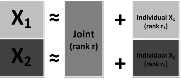
LetX1, X2, ..., Xkbe datatypes on the same set of samples (as in Section 3.1). Variation that is consistent across datatypes in the concatenated matrix X is represented by a singlep×nmatrix of rankr <rank(X). Call this thejoint structure ofX. For eachXi, structured variation in Xi unrelated to the other datatypes is represented by a pi ×n matrix of rank ri < rank(Xi). Call these the individual structure for each Xi. The sum of joint and individual structure gives a low-rank decomposition approximating the dataX. The general model for two datatypes, X1 and X2, is shown in Figure 4.1.

Individual X

1

(rank r

1

)

+

X

₁

Y

≈

Joint

(rank r)

X

₂

Y

≈

₊

Individual X

2

(rank r

2

)

Figure 4.1: Depiction of the JIVE decomposition for two datasets. The data are approx-imated by a low rank matrix of joint variation and low rank matrices giving structured variation unique to X1 and X2.

More formally, let Ji represent the joint structure of Xi, and Ai the individual structure of Xi. Then, the unified model is

X1 = J1+A1 +1

..

. (4.1)

(53)

wherei are pi×n error matrices of independent entries with E(i) = 0pi×n. For J =          J1 J2 .. . Jk         

, A=

         A1 A2 .. . Ak         

the rank constraints require rank(J) =r and rank(Ai) = ri fori= 1, ..., k.

Without further constraints, this decomposition of joint and individual structure is not unique. That is, given J and A1, ..., Ak, there may exist ˜J and Ã1, ...,A˜k of the same ranks such that J 6= ˜J, A 6= Ã, yet J +A = ˜J + Ã. To resolve this issue, we assume that the rows of joint and individual structure are orthogonal:

J AT_i = 0p×pi for i= 1, ..., k.

Intuitively, the orthogonality constraint means sample patterns related to joint variation between datatypes are unrelated to sample patterns responsible for structure in only one datatype. This assumption does not constrain the model, in that any set of datatypes in the form (4.1) can be written equivalently with orthogonality between joint and individual structure. Furthermore, the orthogonality constraint ensures that the joint and individual components in the structure of the concatenated matrixX are uniquely determined. See Appendix A.2 for more details.

Orthogonality of the rows of the individual matrices A1, ..., Ak is not required for the model to be uniquely determined. It is also not explicitly enforced in the estimation of the model (described in Section 4.2). However, imposing this constraint may help to ensure that the Ai matrices are unrelated. This is something we hope to explore in future work.

(54)

4.2 Estimation

Here we discuss estimation of joint and individual structure for fixed ranksr, r1, ..., rk. Section 4.5 discusses the choice of ranks. Joint and individual structure are estimated simultaneously by minimizing the sum of squared error. Let R be the p×n matrix of residual noise after accounting for joint and individual structure:

R=          R1 R2 .. . Rk          =         

X1−J1−A1

X2−J2−A2

.. .

Xk−Jk−Ak

         .

We estimate the model by minimizing the sum of squared residuals ||R||F. This is accomplished by iteratively estimating joint and individual structure:

• FixJ. Find A1, ..., Ak to minimize ||R||F

• FixA1, ..., Ak.Find J to minimize ||R||F

• Repeat until convergence.

Finding joint structure to minimize ||R||F for fixed individual structure is accom-plished by a rank r SVD approximation of X with the individual structure removed. For fixed joint structure, individual structure forXi is found by a rankri SVD approx-imation of Xi with the joint structure removed. The estimate of individual structure forXi will not change that forXj,j 6=i, hence thesek individual SVD approximations minimize||R||F for fixed joint structure. Psuedocode for this iterative approach is given below

• InitializeXJ oint =X = [X₁0 ... X_k0]0

(55)

– Estimate J = [J₁0... J_k0]0 by a rank r SVD approximation of XJ oint

(J =UΛV0)

– For i= 1, ..., k:

∗ Set XIndividual

i =Xi−Ji

∗ Estimate Ai by a rankri SVD approximation of XiIndividual(I−V V0) (Ai =WiΛiVi0)

∗ Set XJ oint

i =Xi−Ai

– Set XJ oint= [X₁J oint0... X_kJ oint0]0

Note that the orthogonality constraint is imposed in the estimation of individual struc-ture. The iterative method is monotone: ||R||F decreases at each step. Hence, ||R||F converges to a coordinate-wise minimum, where it can’t be improved by changing es-timated joint, or individual, structure. Extensive simulations (see e.g., Section 4.7.3) show that the iterative approach appears to minimize the sum of squared residuals in a wide variety of cases. However, a more complete understanding of convergence is desired, and is discussed as future work in Section 4.11.1.

4.3 Relationship to PCA

As in PCA, the rank r joint structure J can be factorized as U S, where U is a p×r

loading matrix andS is an r×n score matrix. Write

(56)

whereUi :pi×r gives the loadings of the joint structure for the rows of Xi. The rank

ri individual structure for Xi can be factorized as WiSi, where Wi is a pi×ri loading matrix andSi is an ri×n score matrix. Then, the low rank decomposition of Xi into joint and individual structure is

Xi ≈UiS+WiSi.

This gives the unified model

X1 = U1S+W1S1+R1

..

. (4.2)

Xk = UkS+WkSk+Rk.

Joint structure is represented by the common score matrix S. These scores elicit patterns in the samples that explain considerable variability across multiple datatypes. The loading matrices Ui indicate how these joint scores are expressed in the rows (variables) of datatype i. The score matrices Si elicit sample patterns individual to datatypei, with variable loadings Wi.

4.4 Dimension Reducing Shortcut

For HDLSS data (pi > n), computing time can be improved by condensing the infor-mation inX1, ..., Xk at the outset. Rather than working with all variables, we consider a dimension-reducing transformation of the original data:

(57)

whereX_i⊥ is n×n. Here, X_i⊥ is derived from an SVD of Xi. If

SV D(Xi) = UiΛiVi0,

thenX_i⊥ = ΛiVi0. Covariance and Euclidian distance between columns (samples) of Xi are preserved in X_i⊥.

Applying the iterative algorithm to the transformed datasets

X⊥=



       

X₁⊥ X₂⊥

.. .

X_k⊥ 

       

can be substantially faster for high-dimensional data. Estimated joint (J_i⊥) and indi-vidual (A⊥_i ) structure for X_i⊥ can then be transformed back to the original variable space through the left singular vectors Ui:

Ji = UiJi⊥

Ai = UiA⊥i .

Applying the iterative estimation method to X directly or estimating joint and individual structure forX_i⊥ and mapping back to the original variable space will yield identical results. Hence, for HDLSS data the data is always transformed via SVD before estimation of joint and individual structure.

Index Catalog // Carolina Digital Repository

Vertical Integration of Multiple High-Dimensional

Datasets

Abstract

Acknowledgments

Table of Contents

List of Figures

List of Tables

Chapter 1

Introduction

1.1

Motivation

1.2

Contributions

1.3

Biological Datatypes

1.4

Applications

1.5

Outline

Chapter 2

Single Multivariate Dataset:

Existing Methods

2.1

SVD

2.2

PCA

2.3

Factor Analysis

Chapter 3

Multiple Datasets: Existing

Methods

3.1

Multi-Block Data

3.2

Pairwise variable associations

3.3

PCA and Factor Analysis of Concatenated Data

3.4

PLS

3.5

O2-PLS

3.6

Canonical Correlation

3.7

Multiple Canonical Correlation

3.8

MF-PCA

Chapter 4

Multiple Datasets: JIVE

4.1

Model

Individual X

(rank r

)

+

X

1

Y

≈

Joint

(rank r)

X

2

Y

≈

+

Individual X

(rank r

)

4.2

Estimation

4.3

Relationship to PCA

4.4

Dimension Reducing Shortcut

₁

₂

₊