COMBINATORIAL INTERPRETATION OF THE KUMAR-PETERSON LIMIT FOR sln(C) DEMAZURE CHARACTERS AND GELFAND PATTERN DESCRIPTION OF
sln(C) DEMAZURE CHARACTERS.
Joseph W. Seaborn III
A dissertation submitted to the faculty at the University of North Carolina at Chapel Hill in partial fulfillment of the requirements for the degree of Doctor of Philosophy in the
department of Mathematics.
Chapel Hill 2014
c
2014
ABSTRACT
JOSEPH W. SEABORN III: Combinatorial Interpretation of the Kumar-Peterson Limit for sln(C) Demazure Characters and Gelfand Pattern Description of sln(C) Demazure
Characters.
(Under the direction of Robert Proctor)
ACKNOWLEDGEMENTS
I would first like to thank my committee. In particular, I would like to thank my advisor Robert Proctor for his guidance in my research and for his substantial help in the writing and editing process. I have learned a great deal through his instruction on both mathematics and exposition.
I would like thank Matt Willis first for discussions and his exposition on his scanning method. His method made the work in this thesis possible. I would also like to thank Matt for helping me edit Chapter 6. I would like to thank David Lax for our numerous discussions on the background and content of this thesis, as well as the related geometry. I would like to thank Allen Knutson and Ezra Miller whose suggestions and insights led to developing the Gelfand pattern scanning method described in Chapter 6.
TABLE OF CONTENTS
LIST OF FIGURES . . . vi
1 Introduction . . . 1
1.1 Overview of thesis . . . 1
1.2 Our combinatorial Kumar-Peterson identity . . . 5
1.3 Demazure tableaux and Willis’ scanning method . . . 8
1.4 Principal specialization and two plane viewpoints . . . 10
1.5 History and hierarchy of generating function identities . . . 11
1.6 Structures for the one columnλ case. . . 12
1.7 Preview of the bijective proof . . . 19
1.8 Geometry and affine labelling tableaux . . . 22
2 Definitions and combinatorial background. . . 25
2.1 n-partitions . . . 25
2.2 Ordered Q-partitions . . . 26
2.3 Inversions of an ordered Q-partition . . . 27
2.4 Reverse semistandard tableaux . . . 28
2.5 Tableau scanning method . . . 29
2.6 Demazure tableaux . . . 30
2.7 Weight monomials and ρ-weight monomials . . . 32
2.8 Weighted limit of a direct system . . . 34
2.9 Labelling tableaux . . . 36
3 Main results . . . 40
3.1 Preliminary results . . . 40
3.3 Main result 2: Our combinatorial K-P identity . . . 45
3.4 Main Result 3: It is a combinatorial interpretation of the K-P identity . . . . 47
4 Bijective proof of our combinatorial K-P identity . . . 48
4.1 Reverse plane partitions . . . 49
4.2 Decomposition of labelling tableaux . . . 49
4.3 Hillman-Grassl board and color template . . . 50
4.4 Template bijection from tableaux to reverse plane partitions . . . 52
4.5 Bijection from labelling tableaux to shrunken labelling tableaux . . . 57
4.6 Bijection from shrunken labelling tableaux to reverse plane partitions . . . . 58
4.7 The colored Hillman-Grassl algorithm . . . 59
4.8 Proof of hook product formula . . . 60
4.9 Decomposition of Φ(ρ). . . 62
4.10 Bijection from multisets of hooks to multisets of shrunken inversions . . . 63
4.11 Bijective proof . . . 65
5 Lie Theoretic proof of combinatorial K-P identity . . . 67
5.1 Transition from Lie theory to combinatorics . . . 67
5.2 Translation of the left hand side . . . 70
5.3 Translation of the right hand side . . . 71
5.4 Lie theoretic proof . . . 72
6 Demazure polynomials from Gelfand patterns . . . 73
6.1 Introduction . . . 73
6.2 Gelfand patterns . . . 74
6.3 Standard bijection from semistandard tableaux to Gelfand patterns . . . 76
6.4 Scanning method for Gelfand patterns . . . 78
6.5 Proofs. . . 86
LIST OF FIGURES LIST OF FIGURES
1 Introduction
The definitions of the combinatorial terms used in this introduction are given in Chapter 2. For the definitions of the Lie theoretic terms used in this thesis, consult Chapter 5. Fix n≥1 throughout this thesis.
1.1 Overview of thesis
Some famous identities in mathematics take the form of a sum equals a product. One such identity is due to Euler: For a nonnegative integer d, denote by p≤n(d) the number of partitions of dwith no more thann parts. Euler described and proved the following product identity for the generating function of these partitions [Sta1]:
∞
X
d=0
p≤n(d)td= 1 n
Y
i=1
(1−ti) .
The Kumar-Peterson (K-P) identity is an identity from Lie theory which is (not obviously) related to this partition generating function identity of Euler. To state the K-P identity, we need to specify 3 inputs: a semisimple Lie (or Kac-Moody) algebraXnof rankn; a dominant integral weightλ which determines a highest weight representationVλ ofXn; and a minimal length coset representative w∈Wλ. Let H be a Cartan subalgebra of Xn. Let Φ be the set of (real) roots ofXn. Let B denote the Borel subalgebra ofXn. LetDλ(w) be the Demazure B-submodule of Vλ with lowest weight w.λ and let dλ(w;y) be the formal character of this submodule with respect to the Cartan subalgebraH. Here the variabley indicates a generic n-variate coordinatization of the ring of formal exponentials of the integral weights for the
coordinatization of the ring of formal exponentials in the simple root basis: For 1≤ i≤ n, we definezi := exp(αi), the formal exponential of the simple rootαi. Define the “adjusted” Demazure character of the Demazure submoduleDλ(w) to bey−wλdλ(w;y). The K-P identity is:
lim m→∞y
−wmλD
mλ(w;y) =
1
Y
α∈Φ(w)
(1−yα) ,
where Φ(w) := Φ+ ∩ w(Φ−). Once the simple root basis has been fixed for the formal exponentials, the adjusted Demazure characters become polynomials in these variables and the right hand sides become formal power series in them. The K-P identity is explicitly stated in the literature only in [Pro1]; there it is indicated how it can be derived from an equation that appeared in the 1996 paper [Kum1] and then later in the book [Kum2].
In this thesis we consider only the TypeAn cases of the K-P identity. So the Lie algebra is sln+1(C).
We introduce combinatorial objects to describe both sides of the K-P identity. Doing so enables us to reformulate the limit on the left side as a sum. The right side remains a product. The easiest cases of the K-P identity occur when the highest weightλis a fundamental weight ωb. Here in Type An, the combinatorial sum equals product identities can be interpreted as product identities for generating functions of reverse plane partitions on general shapes µ. In particular, when the highest weight λ is equal to the fundamental weight ωn, the combinatorial identity can be interpreted as Euler’s partition generating function identity above. The combinatorial translations of the K-P identity for λ = ωb give a Lie theoretic “explanation” of further product identities for reverse plane partition generating functions due to MacMahon [Mac], Stanley [Sta2] and Gansner [Ga]. By describing the K-P identity combinatorially for the general Type An case, we obtain a generalization of this sequence of generating function identities. Our viewpoints also provide explanations for the peculiar colored weighting introduced by Gansner.
λ whose shape we view in the xy-plane. It is well known that the weights of the irreducible representation Vλ can be described with reverse semistandard Young tableaux on the shape λ. We view these reverse semistandard tableaux in the xy-plane. In our combinatorial interpretation of the K-P identity, the limit becomes a sum over a certain set of “labelling tableaux”, which arises when taking the limit. It is interesting to note that this set of labelling tableaux decouples into a direct product of sets of “labelling subtableaux”; this was unexpected. The sets of labelling subtableaux consist of regions of columns of labelling tableaux of the same length. We view these labelling subtableaux in the xy-plane. On the other hand, in some of our combinatorial interpretations and bijective proofs, the tableaux viewed in the xy-plane are transformed via a 3-D picture to reverse plane partitions on a shape µ. As results of this 3-D transformation, both the shape µ and the reverse plane partitions lie in thexz-plane. This shapeµin thexz-plane is the shape on which the reverse plane partitions of MacMahon, Stanley and Gansner are defined.
In 1997, Dale Peterson developed and proved the K-P identity. This identity had already been found independently by Shrawan Kumar. For a poset P, reverse plane partitions generalize to P-partitions. Using the K-P identity, Peterson and Proctor proved [Pro1] that there are hook length product identites for theP-partition generating functions of colored d-complete posets. Shuji Okamura [Oka] and Kento Nakada later gave “Hillman-Grassl-style” bijective proofs of this result for most slant irreducible families of d-complete posets.
By 1990, Lascoux and Sch¨utzenberger [LS] had developed a combinatorial description for Type An Demazure characters. In 2010, Willis developed a simpler method to describe Demazure characters in Type An; this is called the tableau scanning method. His tableau scanning method forms the foundation for the work in this thesis. We first use his notion of “Demazure tableaux” to derive our combinatorial interpretation of the K-P identity from the Lie theoretic K-P identity. Later, in Chapter 6, we also translate Willis’ tableau scanning method to a scanning method for Gelfand patterns. This enables us to describe Demazure characters as sums over Gelfand patterns.
monomials of certain Gelfand patterns. In his proposal, one would define a pipe dream for each Gelfand pattern. One would then convert the pipe dream to a permutation. He proposed that one could describe the Demazure character dλ(w;y) as the sum over the Gelfand patterns whose resulting permutations are weakly less than the permutation w in the Bruhat order. The author of this thesis was not able to describe a method to write Demazure polynomials in this way, but Knutson’s proposal led us to our work in Chapter 6. Jeffrey Ferreira gave [Fe] a description of constituent parts of TypeAn Demazure characters, called “atoms”, as sums over certain Gelfand patterns. We do not, however, address atoms of TypeAn Demazure characters in this thesis.
In the next section, we define a set of tableaux which we call “labelling tableaux”. We then state our combinatorial interpretations of the K-P identity. These are two product identities for a multivariate generating function for the set of labelling tableaux. In Section 1.3, we present Willis’ description of Demazure characters. In Sections 1.4 and 1.5, we describe how the partition and reverse plane partition generating function identities referred to above are special cases of our combinatorial version of the K-P identity. In Section 1.6, we present the various combinatorial and Lie theoretic structures associated to the K-P identity in TypeAn for the case when the highest weight λ is a fundamental weightωn+1−b for some 1 ≤ b ≤ n. Combinatorially, the shape λ obtained from the highest weight λ = ωn+1−b is one column of length b. In Section 1.7, we give a preview of our bijective proof of our first combinatorial interpretation of the K-P identity. In Section 1.8, we present an alternate description of the set of labelling tableaux. We call these tableaux “affine tableaux”. These tableaux provide a better description for the geometric interpretation of the K-P identity.
of the K-P identity for general Type An: the first interpretation gives a generating function identity for the set of labelling tableau in terms of “inversions” of an “orderedQ-partition”; the second gives an identity for the same generating function in terms of “hooks” of “Hillman-Grassl boards”. We then state our third main result, Theorem 3.7 in Section 3.4. This third result states that our first identity in Theorem 3.4 is a combinatorial translation of the Lie theoretic K-P identity for TypeAn. In Chapter 4, we present our bijective proof of Theorem 3.4. In this bijective proof, we use, among other things, Gansner’s colored version of the Hillman-Grassl algorithm. In Chapter 5, we present an alternate proof of the first identity of Theorem 3.4 in which we derive it from the K-P identity by translating Lie theoretic objects into combinatorial objects. In Chapter 6, we present our Gelfand pattern scanning method.
1.2 Our combinatorial Kumar-Peterson identity
To state our combinatorial version of the K-P identity in Type An, we need to specify three inputs: a positive integer n; a subset Q = {q1 < . . . < qk} ⊆ {1,2, . . . , n}; and an “ordered Q-partition” of the set {0,1, . . . , n}:
ρ:={ρn, ρn−1, . . . , ρn+1−q1},{ρn−q1, . . . , ρn+1−q2}, . . . ,{ρn−qk, . . . , ρ0}.
Defineq0 := 0 andqk+1 :=n+ 1. Then for 1 ≤r≤k+ 1, therth block from the left has size
qr−qr−1. We refer to the set of values in each individual block as a “cohort”. Our standard
form for an ordered Q-partition ρ lists the values ρi within each block in decreasing order from left to right:
ρ:= (ρn, ρn−1, . . . , ρn+1−q1;ρn−q1, . . . , ρn+1−q2;ρn−q2, . . .;. . .;ρn−qk, . . . , ρ0).
Q also lists the column lengths that appear in the “labelling tableaux” described below. In Chapter 5, we indicate the equivalence of the ordered Q-partitions ρ in standard form with the minimal length coset representatives w∈Wλ.
For 1 ≤ r ≤ k = |Q|, we define the “ρ-minimal column” Y(r)(ρ) of length q
r to be the vertical column ofqr boxes which contains the leftmostqrvalues inρ, decreasing from top to bottom. In particular, ifQ={b}, for each orderedQ-partitionρthere is only oneρ-minimal column. It has length b and contains the leftmost b values of ρ.
The three combinatorial inputs above determine a set LQ(ρ) of reverse semistandard Young tableaux, which we call “labelling tableaux”. These tableaux T meet the following criteria: the set of distinct column lengths of T is equal to Q; for each 1 ≤ r ≤ |Q| = k, the tableau T has exactly one ρ-minimal column of length qr; and the values in a column appear in the rightmostρ-minimal column to its left. The values in the columns of a labelling tableauT of the leftmost lengthqk are merely bounded below by the values in theρ-minimal column of this length; here the possible values are not restricted to come from a ρ-minimal column to the left.
Note that the values in the region of T of columns of length qr are restricted only by the ρ-minimal columns of length qr and qr+1. Thus the values in the regions of various column
lengths are independent of each other.
combinatorial interpretation of the K-P identity in TypeAnin terms of reverse semistandard tableaux is:”
Theorem 3.4. Fix n ≥ 1, a subset Q ⊆ {1,2, . . . , n}, and an ordered Q-partition ρ. Let Φ(ρ) be the set of inversions of ρ. Then
X
T∈LQ(ρ)
zT = Y 1
(ρi,ρj)∈Φ(ρ)
(1−zρi+1zρi+2. . . zρj)
= k
Y
r=1
Y
(i,j)∈µ(r)
1 1−zhook(i,j).
The “Hillman-Grassl boards” µ(r) here are defined in terms of Q and ρ in Section 4.6.
The hook weightszhook(i,j)are assigned to their boxes in Section 4.3. The weightzT measures T with respect to the tableau of the same shape asT whose columns areρ-minimal columns. Hence we callzT the “ρ-weight monomial” ofT. The variables{zi}n
i=1 that form theρ-weight
monomials correspond to the simple root basis {αi}ni=1.
Note that the first term in the expansion of the right hand side is 1. Given an ordered Q-partitionρ, there is a unique labelling tableau that is formed using one copy of each of the ρ-minimal columns for each of the column lengths in the set Q. This “minimal” labelling
tableau hasρ-weight monomial equal to 1, and is accounted for by the first term of the right hand side. Note that this ρ-weight monomial is not the usual weight monomial for reverse semistandard tableaux; the usual weight monomial only considers the values in a tableauT itself.
Given a subset Q ⊆ {1,2, . . . , n}, there is a “minimal” ordered Q-partition which we denote ρQ0. It is constructed as follows: Form an (n+ 1)-tuple of empty positions. Separate these positions into carrels using semicolons according to the setQ as above. Starting from the left, place the smallest values of {0,1,2, . . . , n} in each cohort. Then, for instance, the values in the leftmost cohort are the numbers {q1−1, q1−2, . . . ,1,0}written in decreasing
order. The simplest cases of our combinatorial identity occur when ρ = ρQ0. In particular, when Q={b} and Q={1,2, . . . , n}, the right hand sides for ρQ0 are respectively
Y
1≤i≤b≤j≤n
1
1−zizi+1. . . zj
and Y
1≤i≤j≤n
1
1−zizi+1. . . zj .
For general Q, the indexing of the product for ρQ0 is over all (i, j) such that there does not exist an r such that qr < i ≤ j < qr+1. The Weyl group element that corresponds to the
orderedQ-partitionρQ0 is the longest element in the setWJ of minimal length representatives, where J :={1,2, . . . , n} −Q.
1.3 Demazure tableaux and Willis’ scanning method
In this section we give a preview of Willis’ recent progress in combinatorially describing Demazure polynomials. It is described in detail for reverse semistandard tableaux in Section 2.5.
We need to first make a technical remark: In the papers [Wi] and [LS] referenced below, permutationsπ ∈Sn and semistandard tableaux were used. However, in the first five chap-ters of this thesis, we use ordered Q-partitions ρ of {0,1,2, . . . , n} instead of permutations and reverse semistandard tableaux instead of semistandard tableaux. The translations from permutations to ordered Q-partitions and from semistandard tableaux to reverse semistan-dard tableaux are given in Chapter 5.
to the weight monomial of λ, coordinatized in the axis basis. Lascoux and Sch¨utzenberger’s [LS] description of Demazure polynomials used the plactic algebra. Their description of Demazure polynomials relied on the construction of the “right key” of a tableau. For a tableau T, the right key R(T) can be defined via a jeu de taquin process, as in Appendix A.5 of [Ful]. The “λ-key of ρ” is the particular key tableau on the shape λ whose columns are ρ-minimal columns. We denote this tableau by Yλ(ρ). Lascoux and Sch¨utzenberger proved thatdλ(ρ;x) is equal to the sum of the weight monomials of the reverse semistandard tableaux T on the shape λ whose right keys satisfy R(T)≥ Yλ(ρ). Following [PW], we say T is a “Demazure tableau” for ρ on the shape λ if R(T)≥ Yλ(ρ). If Dλ(ρ) denotes the set of Demazure tableaux for ρ on the shape λ, then dλ(ρ;x) is equal to the sum of the weight monomials of T ∈ Dλ(ρ). The scanning method developed by Willis simplified the process of finding the right key R(T). Thus his scanning method simplified the description of a Demazure tableau.
We first use the tableau scanning method to describe the limit of the adjusted characters in the left hand side of the K-P identity as a sum over the set of “labelling tableaux”: Fix an orderedQ-partitionρ and letw∈Wλ be the equivalent minimal length representative. The adjusted Demazure polynomials z−wmλD
mλ(w;z) can be expressed as sums of our ρ-weight monomials zT of the Demazure tableaux for ρ. We describe the sets D
mλ(ρ) of Demazure tableaux form≥1 using the scanning method. We then calculate the “set direct limit” of the sequence of sets {Dmλ(ρ)}m≥1. In this limit, the Demazure tableau criterion R(T)≥ Yλ(ρ) simplifies to allow us to label the equivalence classes forming the direct limit with our labelling tableaux. These labels are not necessarily representatives of the equivalence classes, but they do have the same ρ-weight monomial as every member of the equivalence class which they label. We present this transition from limit to sum in our second proof of our combinatorial K-P identity, which is given in Chapter 5.
with top row λ whose scanning pattern entrywise dominates the “λ-key pattern ofπ” to be a “Demazure pattern” for π with top row λ. We prove that the Demazure polynomial for λ and π is equal to the sum of the weight monomials of the Demazure patterns by relating the tableau scanning method to the Gelfand pattern scanning method. We relate the two methods by using the standard bijection from tableaux on shapeλ to Gelfand patterns with top row λ.
1.4 Principal specialization and two plane viewpoints
Theorem 3.4 gives product identities in the n variables zi for a generating function for the set of labelling tableaux. When we coordinatize the K-P identity, the formal exponential of the simple root αi becomes this variable zi. Then the “principal specialization” of our combinatorial K-P identity is produced by setting zi = t for 1 ≤ i ≤ n. Combinatorially, this amounts to ignoring the colors.
Fix an n-partition λand a reverse semistandard tableau T on the shape λ. We vizualize the shape λ in the xy-plane. Consider the following 3-D picture of T: Above the position (i, j) in thexy-plane, stackT(i, j) cubes of side length 1. Move the blocks in the rowx=i up by i−1 positions in the positive z direction. “Project the blocks” to the xz-plane: that is, record the number of blocks in the positive ydirection above each integral position (x, z) in the xz-plane. This produces an upper triangular array of integers in the xz-plane when viewed from the positive y direction, standing on the xy-plane. If we rotate this array 135◦ clockwise we obtain a Gelfand pattern corresponding to T. The top row of this Gelfand pattern is equal to the n-partition λ.
in a column. Note that the indexing (n+ 1−z, b + 1−x) of the rows and columns here is the reverse of the indexing (z, x) provided by the x and z axes. Such an array is called a reverse plane partition on this rectangular shape (bn+1−b). This shape (bn+1−b) should be thought of as lying in the xz-plane.
Letλbe as above. Then Q={b}. Fix an orderedQ-partitionρ. LetT be theρ-minimal column of length b. Convert the column T to a reverse plane partition P on the shape (bn+1−b) as above. Let µ be the shape consisting of the boxes in the rectangle (bn+1−b) with values in P that are equal to 0. This shape µ should also be thought of as lying in the xz-plane. We will see that labelling tableaux for Q = {b} and ρ correspond to the reverse plane partitions on this shape µ. The reverse plane partition generating functions discussed in the next section should be thought of as generating functions for reverse plane partitions on this shape µ.
1.5 History and hierarchy of generating function identities
a special case of MacMahon’s identity when b = 1. By 1971, Stanley [Sta2] had extended MacMahon’s result by obtaining a product identity for the generating function for reverse plane partitions on a general shape µ. Let Q = {b} and let ρ be a general ordered Q-partition; these determine the shape µ in the xz-plane. Stanley’s result now arises as the principal specialization of our K-P identity for this Q and ρ. In 1981, Gansner obtained a multivariate version of Stanley’s identity. He first “colored” the diagonals of the shape µ and then introduced a multivariate weight for a reverse plane partition on µ in terms of these colors. In [Ga], the coloring of the diagonals ofµwas unmotivated. However, when we convert the K-P identity to combinatorics, this coloring process arises naturally. This gives a Lie theory justification for coloring the diagonals as Gansner did. Gansner’s result now arises as our (now unspecialized) combinatorial K-P identity for generalρwithQ={b}. As special cases, both Euler and MacMahon’s identities also have such colored versions. Our identity becomes these colored identities when Q = {1} and Q = {b} respectively and ρ = ρQ0. In 2009, to begin to understand the K-P identity in Type An, Proctor extended MacMahon’s identity by formulating a precursor version of our labelling tableaux for general Q, but only forρ0. Proctor’s tableaux essentially decomposed into k-tuples of reverse plane partitions of
the kind that are handled by the “colored MacMahon” identity. Finally, to view our identity as a generating function for k-tuples of reverse plane partitions, we first construct k shapes
{µ(r)}k
r=1 for the given orderedQ-partition ρ. We then introduce a new set of colors for each
of thesek shapes. By usingk of thexz-plane views as above, our combinatorial K-P identity can be viewed as an identity for the colored generating function ofk-tuples of reverse plane partitions on the k general shapes {µ(r)}k
r=1.
1.6 Structures for the one column λcase
mention most of the combinatorial and Lie theoretic structures that can be associated to this context. We also discuss the shapes that arise in thexz-plane. These are the shapes for the reverse plane partitions of Stanley and Gansner’s generating function identities. Gansner assigned colors to the diagonals of the shape on which he defined his reverse plane partitions. We explain in this section how this peculiar coloring arises. We omit definitions and detailed explanations of the notation used; please refer to Chapters 2 and 5 of this thesis as well as to [Sta1], and [BB], and the appendix of [PW].
Fix 1 ≤ b ≤ n. Let λ be the n-partition (1b) whose shape consists of one column with b boxes. Here Q = {b}. As in Section 1.1, we view this shape λ in the xy-plane. We consider strictly decreasing tableaux on λ with values from {n, n−1, . . . ,0}. Let T be one tableau on the shape λ. Following the procedure in Section 1.4, we obtain a reverse plane partition on the rectangle (bn+1−b) in thexz-plane that corresponds toT. This reverse plane partition consists of only 0’s and 1’s. Converting the 1’s to dots, we can view this reverse plane partition as the Ferrer’s diagram for an (n + 1−b)-partition ν with parts bounded by b. If we replace the 1’s with boxes and rotate 180◦, we obtain a Young diagram ν that fits into the rectangle (bn+1−b). Before the 180◦ rotation, these Young diagrams can also be viewed as order ideals in the product of chains P0 :=(n+1-b)×b. Ordering these by
inclusion produces the distributive latticeJ(P0) that Stanley refers to asL(n+ 1−b, b). The
minimal element of this poset is the empty (n+ 1−b)-partitionν =φ. This partition comes from the tableau T on the shape λ in the xy-plane which has decreasing values from b−1 to 0 down the column. The maximal element of this poset is the full rectangle ν= (bn+1−b). This partition comes from the tableauT on the shapeλin thexy-plane which has decreasing values from n to n+ 1−b down the column.
using piles of blocks on the xy-plane. We shifted these blocks up row by row and projected the y-censuses to the xz-plane. Ignoring the 1’s below the linez =b, we obtained a reverse plane partitionP on the rectangle (bn+1−b). One can see that the 1’s inP along the diagonal colored i arise from values in T which are greater than or equal to i. Thus if a value of T were to be boosted from an i−1 to ani, an additional 1 would be produced in the diagonal colored i. We will see in Chapter 4 that boosting a value i−1 to a value i anywhere in a general tableau T has the effect of multiplying the ρ-weight monomial of both T and P by zi. This corresponds Lie theoretically to adding the simple root αi to the weight ofT, since zi = exp(αi).
Consider a shuffle σ of the (n + 1)-tuple (1b,0n+1−b). Here we index the positions of the (n+ 1)-tuple decreasing from n to 0 from left to right. Recording the positions of the 1’s in a column decreasing from top to bottom produces a column tableau T on the shape λ considered above. The shuffle (1b,0n+1−b) produces the column tableau with maximal values. The shuffle (0n+1−b,1b) produces the column tableau with minimal values. Counting the number of positions that each 1 has moved creates a b-partition µ0 with parts bounded byn+ 1−b. Let µ denote the conjugate of the b-partition µ0; it is an (n+ 1−b)-partition with parts bounded byb. It can be seen that for a given column, its corresponding shapesν andµare “complementary” within the rectangle (bn+1−b). These “Hillman-Grassl boards”µ are the shapes on which the generating functions of Gansner and Stanley are defined; these shapes inherit the colors 1,2, . . . , nfrom the full rectangle (bn+1−b). A shuffle can be viewed as a rearranging operationσ of (n, n−1, . . . ,1,0) such that the values n, n−1, . . . , n+ 1−b and the values n −b, n−b−1, . . . ,1,0 respectively remain in decreasing order. We also index the positions in these (n + 1)-tuples decreasing from n to 0 from left to right. The “inverse shuffle”σ−1 is a rearranging operation of (n, n−1, . . . ,1,0) such that the values in
λ-key ofρby filling the Young diagram of λwith the values in the leftmost cohort ofρ. This is the column tableauT on the shapeλ= (1b) that was produced fromσnear the beginning of this paragraph.
It can be seen that anytime that a new (n+ 1−b)-partitionµ0 bounded byb is produced from µ by appending one box of color i, then in the shuffle picture a 1 in position i was swapped to the right with a 0 from position i − 1. For n ≥ i ≥ 1, let si denote the operation of interchanging the values at positions i and i−1 in an (n + 1)-tuple. Here the symmetric groupSn+1 of rearranging operations on (n+ 1)-tuples can be viewed as the
Weyl group W of Type An acting on its weight spaceEn+1. Re-use the symbol λ to denote the fundamental weight (1b,0n+1−b) = ωn+1−b for sln+1(C). Then the set of shuffles is the
orbit W λ. The stabilizer of λ is the parabolic Weyl subgroup WJ := Wλ = Sb ×Sn+1−b, where J ={1,2, . . . , n} − {n+ 1−b}. Here Sb and Sn+1−b denote the subgroups of Sn+1 of
rearranging operations which rearrange the sets of values within positionsn, n−1, . . . , n+1−b and within positionsn−b, . . .1,0 respectively. Given an orderedQ-partitionρ, view it as an inverse shuffle σ−1. The corresponding σ ∈W is a minimal length representative of a coset
in W/WJ. Let WJ denote the set of such minimal length representatives. Elements of WJ can be labelled with any of the previous structures associated to the column tableaux on the shapeλ. To define the Bruhat order onWJ, view the simple reflections s
i as generators for Sn+1 viewed as a Coxeter group. Now label the elements of WJ with their corresponding
shapes ν. Then the order dual of the Bruhat order on WJ becomes L(n+ 1−b, b). The identity elementσ=eofWJ is depicted as an (n+ 1)-tuple by (n, n−1, . . . ,1,0). Its inverse shuffle σ−1 corresponds to ν = (bn+1−b). The longest element σ = σJ0 of WJ is depicted as an (n+ 1)-tuple by (b−1, b−2, . . . ,1,0, n, n−1, . . . , n+ 2−b, n+ 1−b). Its inverse shuffle σ−1 corresponds to the empty (n+ 1−b)-partition ν =φ.
Return to considering one fixed ordered Q-partition ρfor Q={b}and its corresponding objects σ ∈ W, ν, and µ. Consider the principal filter generated by σ in the order dual of WJ. This produces a lattice which we denote L
P0 that contain ν, ordered by inclusion. Now view the shape µ as a poset whose box at
location (1,1) is its unique maximal element. This is the poset of meet irreducibles of Lσ. We denote this poset Pσ. The ideals of Pσ correspond to reverse plane partitions contained in µ that are bounded by 1. These reverse plane partitions should be viewed as describing “augmentations” ofν in thexz-plane. In the one columnλcase, the (inverse) Hillman-Grassl building procedure produces these reverse plane partitions by adding 1’s to existing reverse plane partitions. The 1’s are added in a manner that corresponds to multiplying by the variables zi = exp(αi).
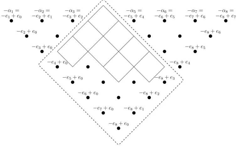
We choose the positive simple roots of Type An to be ei −ei−1 for n ≥ i ≥ 1. For
σ ∈ WJ, set Φ(σ) := Φ+∩σ(Φ−). Then Φ−∩σ−1(Φ+) = σ−1Φ(σ). Let σ0J ∈ WJ be the longest element ofWJ. The set (σJ
0)
−1Φ(σJ
0) of negative rootsβ such thatσ0Jβ ∈Φ+consists
of the negative roots −ej+ei−1 such thatn≥j ≥n+ 1−b≥i≥1. There are b(n+ 1−b)
such negative roots. For an example, take n = 8 and b = 5. These negative roots form the 4×5 rectangle indicated by the dotted line in Figure 1.
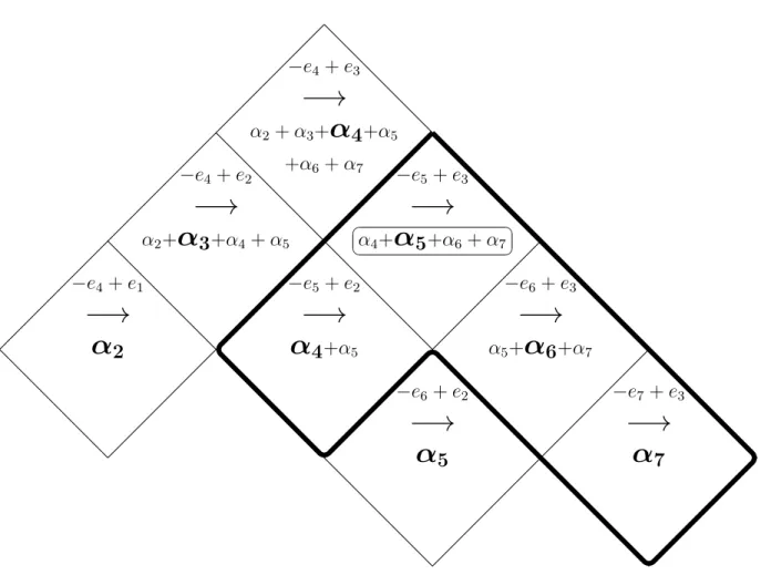
Now fix an orderedQ-partitionρforQ={b}. For example, letρ= (8,6,4,3,1; 7,5,2,0). This determines the corresponding σ ∈ WJ and filter µ ⊆ P0. The corresponding µ is
the shape (4,2,1,0) shown in Figure 2. Since An is simply laced, [Theorem 11, Pro2] (or [Theorem 2.4, BS]) implies that the poset Pσ of join irreducibles is isomorphic to the set of σ−1Φ(σ) of negative roots β such that σ.β ∈ Φ+. So the order structure for our “encompassing Hillman-Grassl board” on which our reverse plane partitions areP-partitions comes from the order structure of the negative roots.
The right hand side of the K-P identity is a product over the positive roots Φ(σ) = σ[σ−1Φ(σ)]. Each positive root α ∈ Φ(σ) can be written as e
ρj −eρi for some “inversion” (ρi, ρj) of ρwherei > j andρi < ρj. The multivariate weight monomial of any such positive root eρj −eρi is zρi+1zρi+2. . . zρj. The colors which we assign to the boxes are indicated inf
Figure 1: Negative roots and the shape µ
−e1+e0 −e2+e1 −e3+e2 −e5 +e4 −e6+e5 −e7+e6 −e8+e7
−α1 = −α2 = −α3 = −α5 = −α6 = −α7 = −α8 =
−e2+e0
−e3+e0
−e4+e0
−e5+e0
−e6+e0
−e7+e0
−e8+e0
−e8 +e1
−e8+e2
−e8+e3
−e8+e4
−e8+e5
−e8+e6
location (1,2) of the shapeµ: One can see that the circled root α4+α5+α6+α7 is equal to
the sum of the colors along the hook at location (1,2) of µ. Thanks to the Hillman-Grassl algorithm, each α ∈ Φ(σ) can be viewed as indicating a potential increment to a colored reverse plane partition on µ: the colors of the augmenting “blocks” must match the colors of the Hillman-Grassl board boxes as the strip of consecutive colors is “wiggled”.
Now let m ≥ 1. The P0-partitions with values bounded by m correspond to the
3-dimensional Ferrers diagrams that fit inside an (n+ 1−b)×b×mbox. These 3-D Ferrers di-agrams arise from the reverse semistandard Young tableaux with possible values{0,1, . . . , n}
on the b×m rectangle in the xy-plane via the stacking, shifting, and truncating process of Section 1.4. MacMahon [Mac] found a quotient-of-products expression for the usual generat-ing function for these P0-partitions. When m= 1, this quotient-of-products is the Gaussian
Figure 2: Hooks on the shape µ
−e4+e3
−→
α2+α3+
α
4+α5+α6+α7 −e 5+e3
−→
α4+
α
5+α6+α7−e6+e3
−→
α5+
α
6+α7−e7 +e3
−→
α
7−e4+e2
−→
α2+
α
3+α4+α5−e5+e2
−→
α
4+α5−e6+e2
−→
α
5−e4+e1
−→
α
2in a Lie theoretic context similar to the context of this thesis. They did this using a de-scription of the highest weight representationVmωn+1−b forsln+1(C) resulting from Seshadri’s standard monomial theorem for minuscule flag manifolds [Se]. There m-multichains in WJ were seen to correspond to the “wedding cake layers” of theP0-partitions at hand. In [Pro2],
the poset P0 and the lattice L(n+ 1−b, b) are respectively viewed as the minuscule poset
an[r] and the minuscule lattice An[r]. Since m was finite, to obtain a product expression identity, it was necessary with the [Pro2] approach to restrict attention to the univariate principal specialization of the Weyl character for Vmωn+1−b. Letting m → ∞ in that result produces the principal specialization of Theorem 3.4 for λ= (1b).
for an irreducible representation of sln+1(C). The corresponding Young diagram λ is the
rectangle (mb) with sole column length b. When λhas only one column length b, it has long been known that the character of the Demazure module ofsln+1(C) with lowest weightρ.λis
described with the reverse semistandard tableaux on the shapeλ which entrywise dominate theλ-key ofρ. Here it is straightforward to form the “direct limit” of the set of such tableaux. This direct limit can be described with the labelling tableaux presented in Section 1.2: In this case these are the reverse semistandard tableaux on the rectangular shapes b×c for c ≥ 1 whose entries are bounded below by the column depiction of ρ and which contain exactly one copy of the column depiction of ρ. Since forming the direct limit commutes with projecting the tableaux to the xz-plane, we can alternatively calculate the direct limit of the set of reverse plane partitions as m → ∞. The direct limit can be described as the set of unbounded reverse plane partitions on the shape µ. Hence the left hand side of the K-P identity may be combinatorially interpreted as the sum of a multivariate weight over these reverse plane partitions.
The two families of Lie theoretic cases which are the most amenable to combinatorial description consist of the TypeA cases and theλ-minuscule cases. This thesis describes the generalization of the [Pro2] situation described above from λ=ωn+1−b,2ωn+1−b,3ωn+1−b, . . . to the general Type A situation for λ,2λ,3λ, . . .. Dale Peterson independently developed the K-P identity to help Proctor obtain [Pro1] the generalization from the [Pro2] cases toP -partitions on alld-complete posets; this generalization used theλ-minuscule representations of the simply-laced Kac-Moody algebras.
1.7 Preview of the bijective proof
In this section we present a preview of the bijective proof of our combinatorial interpre-tation of the K-P identity, Theorem 3.4.
The left hand side, as originally stated, is a sum over the labelling tableaux:
X
T∈LQ(ρ) zT.
As we noted in Section 1.2, the values in a labelling tableau in each region of a distinct column length are independent from the values in the regions of a different column length. This enables us to write the set of labelling tableaux as a Cartesian product of k sets, denoted L(Qr)(ρ) for 1 ≤ r ≤ k. The set L(Qr)(ρ) consists of the tableaux T(r) such that the
only column length for T(r) is qr, the values of T(r) come from the ρ-minimal column of length qr+1, and T(r) contains exactly 1 ρ-minimal column of length qr. These tableaux appear as “subtableaux” of the labelling tableaux. We can then write LQ(ρ) =
k
Y
r=1
L(Qr)(ρ). This enables us to rewrite the sum on the left hand side as
k
Y
r=1
X
T∈L(Qr)(ρ)
zT
.
Starting with r = k and proceeding tor = 1, we produce k identities that equate these factors of the left hand side to k products over certain subsets of inversions of ρ. When r = k, we construct a shape µ(k) which we call a “Grassl board”. This
Hillman-Grassl board is defined by the values in the ρ-minimal column of length qk. Here the shape µ(k) is constructed from the ordered Q-partition ρ as in Section 1.4. We now “color” the diagonals ofµ(k). For now, each color is a one element subset of{1,2, . . . n−1, n}. Forr < k,
each new “composite” color will be a subset of consecutive integers of {1,2, . . . , n−1, n}. Now we construct three weight-preserving bijections. For our first bijection when r=k, we map tableaux in the set L(Qk)(ρ) to reverse plane partitions on the shape µ(k). This map is
we use the opposite direction. That is, for our second weight-preserving bijection, we use the colored Hillman-Grassl algorithm to map reverse plane partitions on µ(k) to the set of
multisets of “hooks” on µ(k). To set up our third weight-preserving bijection, we construct a map from the set of hooks of µ(k) to a certain subset of the set Φ(ρ) of inversions of ρ.
We denote this subset by Φ(k)(ρ). This induces our third weight-preserving bijection: a map
from the set of multisets of hooks ofµ(k) to the set of multisets of elements of the set Φ(k)(ρ). Denote by M Φ(k)(ρ) the set of multisets of elements of Φ(k)(ρ). These three bijections give us the following identity:
X
T∈L(Qk)(ρ)
zT = X
S∈M(Φ(k)(ρ))
zS.
The current right hand side of this identity is the naive expansion of
1
Y
(ρi,ρj)∈Φ(k)(ρ)
(1−zρi+1zρi+2. . . zρj) .
Thus we have
X
T∈L(Qk)(ρ)
zT = Y 1
(ρi,ρj)∈Φ(k)(ρ)
(1−zρi+1. . . zρj) .
Now for k −1 ≥ r ≥ 1, we similarly construct Hillman-Grassl boards µ(r). For fixed k−1≥r≥1, these Hillman-Grassl boards are constructed from the values in theρ-minimal columns of length qr and qr+1. However, we need to carefully form the colors for these
boards. The colors assigned to the diagonals of the Hillman-Grassl board µ(r) are formed from unions of colors that were assigned to the boardµ(r+1). Fork−1≥r≥1, we construct
subsets Φ(r)(ρ)⊂Φ(ρ). Then fork−1≥r ≥1, we define three weight-preserving bijections
as above. For k−1≥r≥1, these three bijections give us the following identities:
X
T∈L(Qr)(ρ)
zT = Y 1
(ρi,ρj)∈Φ(r)(ρ)
Finally, the proof can be completed with the observation that Φ(ρ) =tk r=1Φ
(r)(ρ). Thus we
have
X
T∈LQ(ρ) zT =
k Y r=1 X
T∈L(Qr)(ρ)
zT = k Y r=1 1 Y
(ρi,ρj)∈Φ(k)(ρ)
(1−zρi+1. . . zρj)
= Y 1
(ρi,ρj)∈Φ(ρ)
(1−zρi+1. . . zρj) .
1.8 Geometry and affine labelling tableaux
Here we present another choice of tableaux for labelling the equivalence classes that arise when we form the weighted limit of the sequence of sets of Demazure tableaux. The specification of these tableaux is only slightly different from the definition of the labelling tableaux presented in Section 1.2; this formulation is more closely related to the geometric structures that provided the original context for the Kumar-Peterson identity.
Fix a subset Q ⊆ {1,2, . . . , n} and an ordered Q-partition ρ. For 1 ≤ r ≤ k, recall that the ρ-minimal column of length qr is the vertical column of qr boxes which contains the leftmost qr values inρ, decreasing from top to bottom. This column is denoted denoted Y(r)(ρ). We define the set of affine labelling tableaux to be the tableaux T which meet the following criteria: each column length of T is in Q; the allowable columns of length qr are those which dominate but do not equal Y(r)(ρ) ; and the values in the columns of length qr come from the ρ-minimal column Y(r+1)(ρ). To convert a labelling tableau S to the corresponding affine labelling tableau T, delete the one copy of each ρ-minimal column from S. Note that the null tableau∅ is an affine labelling tableau for every choice of n, Q, and ρ.
Example 1.1. Fixn = 2,Q={1}, andρ=ρQ0 = (0; 2,1). The ρ-minimal column of length 1 is 0 . Here the labelling tableaux are
The affine labelling tableaux are
∅ , 1 , 2 , 1 1 , 2 1 , 2 2 , . . . .
These affine labelling tableaux can be obtained from the labelling tableaux by deleting the ρ-minimal column 0 from each tableau respectively.
The Q = {1} and ρ = ρQ0 case of our work provides a combinatorial model for the usual realization of affine n-space within projective n-space: Set V :=Cn+1. Let f0, . . . , fn
denote the axis basis for V∗. These are global sections on Pn :=
P(V) for its standard line
bundle. The homogeneous coordinate ring for Pn is M m≥0
SmV∗. Here SmV∗ consists of the homogeneous polynomials of degree m in the fi. The group GL(n+ 1) acts on V∗ via the contragredient of the natural representation. Its torus subgroup T consists of the diagonal matrices t := (t0, . . . , tn). Define characters xi : T → C∗ by xi(t) := t−i 1. The character of T under the induced action of GL(n+ 1) onSmV∗ is the homogeneous symmetric function hm(x0, . . . , xn). This may be depicted with the (n+ 1)-reverse semistandard Young tableaux (defined in Section 2.4) on the one row shape (m1). The affine space An may be realized within Pn by requiring that f0 = 1. Its affine coordinate ring is R := C[f1, . . . , fn]. Here
the character for the induced action of T on R is the sum of all monomials in f1, . . . , fn. This may be depicted with the one row affine labelling tableaux, as in the example above for n= 2: Here the value i in a tableau is to be interpreted as the variable xi, and so these tableaux depict the monomials 1, x1, x2, x21, x1x2, x22, . . ..
The Q = {b} and general ρ case of our work provides a combinatorial model for the affine coordinate ring of a Bruhat cell within the Grassman manifoldGb,n+1: Here the global
sections on all of Gb,n+1 of its standard line bundle are certain b×b “minor” polynomials
that are formed from certain variables that are drawn from an (n+ 1)×barray of variables; for projective space the f0, . . . , fn were 1×1 minor polynomials drawn from the column of
These minors are depicted by the (n+ 1)-reverse semistandard Young tableaux on the one column shape (1b). Fix an orderedQ-partition ρ and consider the corresponding ρ-minimal columnY(1b)(ρ). The Schubert subvariety ofGb,n+1 indexed byρ is determined by setting to zero the minors that are indexed by the one column tableaux that do not dominate Y(1b)(ρ). Here a basis for the space of global sections of degreemfor the standard line bundle restricted to the subvariety can be obtained by choosing them-fold products of minors that are indexed by the (n+ 1)-reverse semistandard Young tableaux on the shape (mb) which are comprised of the “surviving” columns. The corresponding Bruhat cell arises when the minor indexed byY(1b)(ρ) is set equal to 1. The character for the action ofT on the affine coordinate ring of this cell is the sum of our weight monomialsxT over the affine labelling tableaux forQ={b}
and ρ. Here the shapes of the affine labelling tableaux are all the rectangular shapes with b rows along with the empty shape (which can be viewed as the shape with b rows and no columns.) Here the exclusion of the ρ-minimal column from the affine labelling tableaux corresponds to setting this minor to 1.
LetQbe arbitrary. This specifies a certain flag manifold of TypeAn. Choosing an ordered Q-partition ρ specifies a Schubert subvariety. David Lax has used Willis’ scanning method to simplify Reiner’s and Shimozono’s Demazure tableaux derivation of bases of “standard monomials” of minors for the spaces of global sections of the standard line bundles [Lax]. Here the Bruhat cell indexed byρ arises when the product of the minors that correspond to the ρ-minimal columns is set to 1.
2 Definitions and combinatorial background
In this chapter, we introduce the combinatorial structures needed to state our main results in Chapter 3. In Sections 2.1 to 2.3, we define n-partitions, ordered Q-partitions, and inversions of ordered Q-partitions. The first right hand side of our second main result, Theorem 3.4, is a product over the inversions of an ordered Q-partition; the second right hand side is a product over the “hooks” of certain “Hillman-Grassl boards”. We define the boards in Section 4.6. In Section 2.4 we introduce reverse semistandard tableaux. In Section 2.5, we present Willis’ tableau scanning method in terms of reverse semistandard tableaux. This allows us to give our definition of Demazure tableaux in Section 2.6. In Section 2.7, we define the usual weight monomial of a tableau and the ρ-weight monomial of a Demazure tableau. These monomials constitute the terms of the Demazure polynomials and “adjusted” Demazure polynomials respectively. We give a definition of the “weighted limit” of a direct system of sets equipped with maps in Section 2.8. Finally, in Section 2.9, we define the set of labelling tableaux.
2.1 n-partitions
Denote the set of integers from 1 to nby [n] and the set of integers from 0 ton by [0, n]. For integersi < j, define (i, j] :={i+ 1, . . . , j}, and [i, j) :={i, . . . , j−1}. An n-partition λ is ann-tuple (λ1, λ2, . . . , λn) of integers such thatλ1 ≥λ2 ≥. . .≥λn≥0. Fix ann-partition
λ. For m ≥ 1, define mλ := (mλ1, mλ2, . . . , mλn). The Young diagram (or shape) λ, also denoted λ, consists ofλi left justified boxes in theith row for 1≤i≤n. Let (i, j) denote the box in the ith row and thejth column in λ. For 1 ≤j ≤ λ1, let ζj be the number of boxes
in the jth column in λ. Let k denote the number of distinct column lengths inλ. Denote the set of distinct column lengths of λ by Q(λ) := {q1, q2, . . . , qk}, where qi < qi+1. Note
mλhave the same set of distinct column lengths.
2.2 Ordered Q-partitions
Fix an integer 1≤k ≤n. Let Q={q1, q2, . . . , qk} be a subset of [n] such thatqi < qi+1.
We define an ordered Q-partition ρ to be a partition of the set [0, n] into k+ 1 parts such that the rth part has size qr−qr−1 for 1≤r≤k+ 1. We notate ρas an (n+ 1)-tuple
(ρn, ρn−1, . . . , ρn+1−q1;ρn−q1, . . . , ρn+1−q2;ρn−q2, . . .;. . .;ρn−qk, . . . , ρ0),
where the parts are separated by semicolons. The standard form of ρ is the unique such (n+ 1)-tuple whose entries decrease from left to right within each part. Throughout this thesis, we assume that orderedQ-partitions are in standard form. Denote the set of ordered Q-partitions bySnQ+1. We call the set of positions (values) within each part acarrel (cohort). So the number of carrels (cohorts) in ρ∈SnQ+1 is k+ 1.
The orderedQ-partition ρin standard form will play the role in our interpretation of the K-P identity that the minimal length representative w ∈ WJ plays in the Lie theory K-P identity, whereJ := [n]−Q. We show in Chapter 5 how to obtain an ordered Qpartition ρ fromw.
Given an ordered Q-partitionρ, we define aQ-chain of ordered subsets B1 ⊂B2 ⊂. . .⊂
Bk+1 by Bi :=Bi,ρ :={ρn, ρn−1, . . . , ρn+1−qi}. So the set Bi contains the leftmost qi entries of ρ. Henceforth the elements of Bi are to be listed in decreasing order from left to right. Note that Bk+1 = [0, n]. We define B0 = ∅. For 1≤ i≤ k+ 1, we denote the ith cohort of
ρ by Hi. Note that we have Hi = Bi\Bi−1 and Bi = H1 tH2 t. . .tHi for 1 ≤i ≤k+ 1. DefineBi(j) and Hi(j) to be the jth largest entries ofBi and of Hi respectively.
the same combinatorial identity. For this reason, in our identity, we take the set Q as our starting point instead of λ.
Example 2.1. Fixn = 8. Letλbe the 8-partition (1,1,1,1,1,0,0,0). Here λ has just one column of length 5. Hence Q:=Q(λ) ={5}. Since Q contains k = 1 integer, there are two cohorts for any ordered Q-partition ρ∈S9Q. Consider ρ= (7,6,4,2,1; 8,5,3,0)∈S9Q. Here ρ8 = 7 and ρ0 = 0. The Q-chain of subsets produced from ρ is B1 ={7,6,4,2,1} ⊂ B2 =
{8,7,6,5,4,3,2,1,0}. Here we haveH1 ={7,6,4,2,1} and H2 ={8,5,3,0}.
Example 2.2. Fix n = 9. Let λ be the 9-partition (4,4,2,2,1,1,1,0,0). We have Q := Q(λ) = {2,4,7}. Since Q contains k = 3 integers, each ρ ∈ S10Q has four cohorts. Let ρ= (5,1; 8,4; 9,3,0; 7,6,2); here ρ∈S10Q and fromρ we produce the Q-chain of subsets
{5,1} ⊂ {8,5,4,1} ⊂ {9,8,5,4,3,1,0} ⊂ {9,8,7,6,5,4,3,2,1,0}.
We then have, for example, B3(2) = 8.
2.3 Inversions of an ordered Q-partition
An inversion of an ordered Q-partition ρ is defined to be an ordered pair (ρi, ρj) such that i > j and ρi < ρj. That is, an inversion is a pair of values in the (n+ 1)-tuple ρ which increase from left to right. Note that no inversion can consist of a pair of values in the same cohort since the values in each cohort decrease from left to right. Denote the set of inversions of ρ by Φ(ρ). The right hand side of the generating function identity in Theorem 3.4 is a product over the set of inversions of an ordered Q-partition ρ.
Example 2.3. Fix n = 8. As in Example 2.1, let Q = {5} and ρ = (7,6,4,2,1; 8,5,3,0). The set of inversions of ρ is
Example 2.4. Fixn= 9. As in Example 2.2, letQ={2,4,7}andρ= (5,1; 8,4; 9,3,0; 7,6,2). Here we have
Φ(ρ) = {(5,7),(1,7),(4,7),(3,7),(0,7),(5,6),(1,6),(4,6),(3,6),(0,6),
(1,2),(0,2),(5,9),(1,9),(8,9),(4,9),(1,3),(5,8),(1,8),(1,4)}.
Let z1, z2, . . . , zn be variables. We define theweight monomial of an inversion (ρi, ρj) to be zρi+1zρi+2. . . zρj =:z(ρi,ρj].
Givenρ ∈SnQ+1, in Section 4.9 we decompose the set of inversions ofρintok =|Q|disjoint subsets. This decomposition will form a crucial step in the bijective proof of Theorem 3.4.
2.4 Reverse semistandard tableaux
Fix ann-partitionλ. Areverse(n+1)-semistandard tableau T on the shapeλis a filling of the shapeλ with elements from [0, n] such that the valuesT(i, j) satisfyT(i, j)≥T(i, j+ 1) and T(i, j) > T(i+ 1, j) whenever both values are defined. Denote the shape of T by shape(T). Let Tλ denote the set of all reverse (n+ 1)-semistandard tableaux on the shape λ. We refer to a reverse (n+ 1)-semistandard tableau simply as a tableau. For 1≤j ≤λ1,
letTj denote thejth column of T. If the shape λ consists of only one column, then we refer to a tableau on the shape λ as a column. If λ = (0,0, . . . ,0) is the n-partition consisting of all 0’s, then we refer to the shape λ as the empty shape, denoted φ. This shape φ does not contain any boxes. There is a unique tableau on the shape φ which we call the null tableau. Since the empty shape contains no boxes, the null tableau contains no values. ForT, U ∈ Tλ, write T ≤ U if T(i, j) ≤ U(i, j) for all (i, j) ∈ λ. A tableau is a key if all the values in a column also appear in every column to the left of that column.
As noted earlier, the n-partition λ determines a subset Q⊆[n] and an integer k :=|Q|. Now fix an ordered Q-partition ρ ∈ SnQ+1. This determines the Q-chain of subsets B1 ⊂
placing the values of Br in descending order from top to bottom. We denote the value in Yλ(ρ) in position (i, j) by Yλ(ρ;i, j). So Yλ(ρ;i, j) = Br(i) if ζj = qr. Note that any two columns of Yλ(ρ) of the same length are equal. For 1 ≤ r ≤ k, we call a column of length qr the ρ-minimal column of length qr if it appears as one of these equal columns in Yλ(ρ) of length qr. Denote this ρ-minimal column of length qr by Y(r)(ρ). Note that the number of columns in λof length qr is equal toλqr+1−λqr for 1≤r ≤k. So Yλ(ρ) containsλqr−λqr+1
columns equal to Y(r)(ρ) for 1≤r≤k.
Example 2.5. Fix n = 9. Let λ = (4,4,2,2,1,1,1,0,0) and ρ = (5,1; 8,4; 9,3,0; 7,6,2)∈
S10Q as in Example 2.2. Here Q={2,4,7} and
Yλ(ρ) =
9 8 5 5 8 5 1 1 5 4 4 1 3 1 0
.
The three ρ-minimal columns in this case are
Y(3)(ρ) = 9 8 5 4 3 1 0
, Y(2)(ρ) = 8 5 4 1
, Y(1)(ρ) = 5 1 .
2.5 Tableau scanning method
Fix an n-partition λ. LetT ∈ Tλ. In this section we construct thescanning tableau S(T) of T using the scanning method developed by Willis [Wi]. The tableau scanning method is defined in [Wi] in terms of semistandard tableaux. However, here we state its analog for reverse semistandard tableaux.
We need the following preliminary definition: Given a sequence (s1, s2, s3, . . .), its earliest
index ij is the smallest index such thatsij−1 ≥sij.
Given T ∈ Tλ, construct the scanning tableau S(T) as follows: Draw an empty Young diagram of the shape λ. Viewing the bottom values of the columns of T from left to right as forming a sequence, find the EWDS of this sequence. Whenever a value is added to the EWDS, put a dot above it. When this EWDS ends, write its last member in the diagram for the scanning tableau of T in the lowest available box in the leftmost available column. Repeat the process as if the boxes with the dots and the values in them are no longer a part of T. Once every box in T has a dot, the leftmost column of the right key has been formed. To find the values of the next column in the right key: ignore the leftmost column of T, erase the dots in the remaining boxes, and repeat the above process. Continue in this manner until the Young diagram has been filled with values; this is the scanning tableau S(T) of T.
The right key ofT, denotedR(T), is a special key tableau that is defined in e.g. Section 3 of [RS]. By the main result Theorem 2.5.5 of [Wi], we know that R(T) =S(T). Thus the scanning method gives a direct description of R(T), and in this thesis we calculate the right key ofT using only the scanning method. We denote the value inR(T) at position (i, j) by R(T;i, j). It is a known result, stated in Corollary 3.4 of [PW], that T ≥R(T) =S(T).
2.6 Demazure tableaux
Demazure tableaux are defined in [PW] for n-semistandard tableaux. Here a reverse (n+ 1)-semistandard tableau T on the shape λ is defined to be a Demazure tableau for ρ if R(T)≥Yλ(ρ). The set of Demazure tableaux for ρ on the shape λ is denoted Dλ(ρ).
are two tableaux on the shape λ:
T =
9 9 8 6 8 6 2 1 6 5 5 2 3 2 1
, U =
9 8 4 3 8 4 2 1 6 3 4 1 3 2 0 .
We use the scanning method to construct the right keys of these tableaux:
R(T) =
9 8 6 6 8 6 1 1 6 5 5 1 3 2 1
, R(U) =
9 8 3 3 8 3 1 1 6 2 3 1 2 1 0 .
We now consider an ordered Q-partition ρ and determine if Dλ(ρ) contains T and/orU from Example 2.6:
Example 2.7. Fix n = 9 and λ as in Example 2.6. Let ρ = (5,1; 8,4; 9,3,0; 7,6,2)∈ S10Q. The λ-key of ρ was constructed in Example 2.5. For all (i, j) ∈ λ, we have R(T;i, j) ≥
Yλ(ρ;i, j). Hence T is a Demazure tableau for ρ of shape λ. The tableau U is not a Demazure tableau for ρ since, for instance, we have R(U; 1,3) = 3<5 = Yλ(ρ; 1,3).
Calculating the set of Demazure tableaux is particularly simple when λ consists of just one column:
Example 2.8. Fixn= 8 andλ= (1,1,1,1,1,0,0,0,0). Letρ= (7,6,4,2,1; 8,5,3,0)∈S9Q. Then the λ-key of ρ is the following:
Yλ(ρ) = 7 6 4 2 1 .
by calculating the right keys of the tableaux T ∈ Tλ via the scanning method. However, it can be seen that R(T) = T for any column tableau. Hence with this particular λ, we have R(T) ≥Yλ(ρ) if and only if T ≥ Yλ(ρ). So the set of Demazure tableaux Dλ(ρ) here is the set of tableau on the shapeλ with values from [0,8] which are entrywise greater thanYλ(ρ). The entrywise smallest such tableau is
7 6 4 2 1 .
The entrywise largest such tableau is
9 8 7 6 5
.
2.7 Weight monomials and ρ-weight monomials
Fix ann-partitionλand an orderedQ-partitionρ. In this section we define weight mono-mials for reverse semistandard tableaux andρ-weight monomials for Demazure tableaux. Let x0, x1, . . . , xn be variables. GivenT ∈ Tλ, itsweight monomial is defined to bexT :=
n
Y
i=0
xcii , where ci is the number of times the value i occurs in T. This is the traditional weight monomial of a tableau.
Example 2.9. Let T be the tableau in Example 2.6. Here we have xT =x2
9x28x36x52x3x32x21.
Letλbe ann-partition andρ∈SnQ+1 be an orderedQ-partition. A certainkey polynomial kρ,λ(x) is defined in [PW] and [RS] by applying a sequence of divided difference operators to the weight monomial of the tableau on λ with the largest possible values. According to Theorem 1 of [RS] we have
Theorem 2.10.
kλ,ρ(x) =
X
We define the Demazure polynomial for λ and ρ to be dλ(ρ;x) :=
X
T∈Dλ(ρ) xT.
Introduce variablesz1, z2, . . . , znbyzi :=xi−−11xi. Given T ∈ Dλ(ρ), we define itsρ-weight
monomial to be zT := xYλ(ρ)−1
xT. We write the ρ-weight monomials in terms on the variables zi.
Note that the ρ-weight monomial of T depends onρ and T, while the weight monomial depends only on T. Further, the adjusted weight monomial is only defined for Demazure tableaux.
We now calculate the ρ-weight monomial of the tableau T from Example 2.6:
Example 2.11. Fix n = 9. As in Example 2.5, let λ = (4,4,2,2,1,1,1,0,0) and ρ = (5,1; 8,4; 9,3,0; 7,6,2)∈S10Q. LetT be the tableau in Example 2.6. Theρ-weight monomial of T is given by
zT = x T xYλ(ρ) =
x29x28x36x25x3x32x21
x9x28x45x24x3x41x0
= x9x
3 6x32
x2
5x24x21x0
=z1z23z 2 5z
4
6z7z8z9.
Given λand ρ, we define the adjusted Demazure polynomial to beDλ(ρ;z) := X T∈Dλ(ρ)
zT. We then obviously have the relationship Dλ(ρ;z) = xYλ(ρ)
−1
dλ(ρ;x). It will be seen in Lemma 2.12 that the adjusted Demazure polynomials are actually polynomials in the zi variables.
Fix T ∈ Tλ. Let C be a column of T of length qr for some 1 ≤ r ≤ k. The ρ-weight monomial of C is zC :=xY(r)(ρ)−1xC. Note that zT =Y
C
zC, where the product is over the columns C of the tableau T. We use this method to calculate the ρ-weight monomials of the “labelling tableaux” later in this chapter. Calculating the ρ-weight monomials of Demazure tableaux in this way, we see that ρ-minimal columns play a special role in the ρ-weight calculation:
have nonnegative exponents.
Proof. SupposeC is a column ofT of lengthqr which is not equal toY(r)(ρ). For 1≤i≤qr, letC(i) andY(r)(ρ;i) denote the values in row i of columns C and Y(r)(ρ) respectively. We can calculate the ρ-weight of the column C as a product over the individual boxes of C as follows:
zC =xY(r)(ρ) −1
xC = qr
Y
i=1
xY(r)(ρ;i)
−1
xC(i).
Recall that we have T ≥R(T) ≥Yλ(ρ). Then the column C must satisfy C(i) ≥ Y(r)(ρ;i) for all 1 ≤i ≤ qr. Since C 6= Y(r)(ρ), for some 1 ≤ i≤ qr, we must have C(i)> Y(r)(ρ;i). This valueC(i) contributes xY(r)(ρ;i))
−1
xC(i) =zY(r)(ρ;i)+1zY(r)(ρ;i)+2. . . zC(i) to theρ-weight
of C. Also, since C(i) ≥ Y(r)(ρ;i) for all 1 ≤ i ≤ qr, no value of C contributes a negative power of any zt variable for 1 ≤ t ≤ n. Hence a column which is not a ρ-minimal column contributes at least onezt factor to theρ-weight monomial ofC. On the other hand, clearly any ρ-minimal column contributes only a factor of 1 to the ρ-weight monomial of T. Since every column contributes a nonnegative factor of somezi variable, clearlyzT is a product of the zi variables with nonnegative exponents.
2.8 Weighted limit of a direct system
A set ofweighted combinatorial objects is a finite setB of combinatorial objects equipped with a function wt : B → Nn. Given b ∈ B we refer to wt(b) as the weight of b. Suppose wt(b) = (t1, t2, . . . , tn). Define the weight monomial of b to be zb := zwt(b) := z1t1z
t2
2 . . . zntn. We define |wt(b)| := t1 +t2 + . . .+tn. The generating function for B is defined to be FB(z) :=
X
b∈B
zb. This polynomial is an element ofC[[z1, z2, . . . , zn]], the ring of formal power series in the variables z1, z2, . . . , zn.
Define a relation ∼ on the elements of the set A := G m≥1
Am as follows: Let a, b ∈ A. Define a∼b if there exists 1≤ i≤j such that a ∈Ai and b ∈Aj and φi,j(a) =b or b ∈Ai and a∈Aj and φi,j(b) = a. This is an equivalence relation on A. We define the limit of the direct system ({Am},{φi,j}) to be the set A/∼of equivalence classes E of ∼.
Let E ∈ A/ ∼. It can be seen that E is a set of elements from consecutive sets Am: Injectivity implies that we can writeE ={at, at+1, at+2, . . .}for somet≥1 such that ai ∈Ai for i≥t.
Now suppose the sets Am in the direct system ({Am},{φi,j}) are equipped with weight functions wt :Am →Nn. For each ν ∈ Nn, denote by Am,ν the subset of Am of elements of weight ν. We refer to this structure ({Am},{φi,j}, wt) as a weighted direct system of sets. Let E ∈ A/∼. We say that E is a tame class if there exists a weight ν ∈Nn and M
E ≥1 such that for all i ≥ ME, we have wt(ai) = ν. In this case we define wt(E) := ν and zE := zν. We define the weighted limit of the weighted direct system ({A
m},{φi,j}, wt) to be the subset of tame classes in A/ ∼. We denote this weighted limit by lim
m→∞(Am, φ, wt). We call a weighted limit of a weighted direct system stable if for every weight ν ∈Nn, there existsfν ≥0 and Mν ≥1 such that the number of tame classes of weight ν in the weighted limit is equal tofν and form≥Mν, we have|Am,ν|=fν. We define the generating function of a stable weighted limit of a weighted direct system ({Am},{φi,j}, wt) to be
F lim
m→∞(Am, φ, wt)(
z) := X
E∈ lim
m→∞(Am, φ, wt) zE.
Given a formal power seriesF(z) andν ∈Nn, define< F(z), ν >to be the coefficient ofzν inF(z). Note that for a setAm of weighted combinatorial objects, we have < FAm(z), ν >=
|Am,ν|. A sequence of multivariate polynomials {FAm(z)}m≥1 is said to converge to a formal
power series F(z) as m → ∞ if for each ν ∈ Nn there exists L
ν such that for m ≥ Lν, we have< FAm(z), ν >=< F(z), ν >. Then this limit is denoted lim
Lemma 2.13. If the weighted limit asm→ ∞of the weighted direct system({Am},{φi,j}, wt) is stable, then
lim
m→∞FAm(z) = F lim
m→∞(Am, φ, wt)( z),
where the limit on the left hand side is found in the ring of formal power series.
Proof. Fix some ν ∈ Nn. Since the weighted limit is stable there exists fν ≥ 0 such that the number of tame classes of weightν in the weighted limit is equal tofν. That is, we have < F lim
m→∞(Am, φ, wt)(
z), ν >=fν. Also from the stability of the weighted limit, there exists anMν ≥1 such that for m≥Mν, we have< FAm(z), ν >=|Am,ν|=fν. Now let Lν :=Mν. Then clearly for m ≥ Lν, we have < F lim
m→∞(Am, φ, wt)(
z), ν >=< FAm(z), ν >. Thus the polynomials FAm(z) converge to the formal power seriesF lim
m→∞(Am, φ, wt)( z).
From this lemma, we know that if the weighted limit of a weighted direct system is stable, then the limit of the generating functions of the sets exists in the ring of formal power series. Once we know the weighted limit is stable, it may be useful to label the equivalence classes of the weighted limit with objects from a (not necessarily finite) set B of weighted combinatorial objects. We do so by defining a map Ψ : lim
m→∞(Am, φ, wt)→ B. We call this ordered pair (Ψ,B) a labelling of lim
m→∞(Am, φ, wt) if Ψ is injective and wt(Ψ(E)) = wt(E) for all equivalence classes E ∈ lim
m→∞(Am, φ, wt). Elements of Ψ( limm→∞(Am, φ, wt)) are called the labels of the equivalence classes of the weighted limit.
2.9 Labelling tableaux
Re-fix an n-partition λ and an ordered Q-partition ρ. For 1≤r≤ k, we define gr to be the number of columns of length qr in the shape λ. Note that we havegr =λqr −λqr+1.