ISSN: 1311-1728 (printed version); ISSN: 1314-8060 (on-line version) doi:http://dx.doi.org/10.12732/ijam.v33i4.5
A GENERALIZED FINITE-DIFFERENCES SCHEME USED IN MODELING OF A DIRECT
AND AN INVERSE PROBLEM OF ADVECTION-DIFFUSION
F. Dom´ınguez-Mota1§, J.S. Lucas-Mart´ınez2, G. Tinoco-Guerrero3 1,2,3 F.C.F.M, U.M.S.N.H
Francisco J. M´ujica S/N Morelia - 58030, MEXICO
Abstract: This work presents the use of a schemes in generalized finite-differences for the calculation of a numeric solution associated to a stationary, advection-diffusion problem, and the usage of such schemes in the study of an inverse problem related to this one, in which a non-linear, regularized least-squares adjustment is employed to determine certain coefficients involved in the problem.
AMS Subject Classification: 75N06, 65M50, 74S20
Key Words: generalized finite difference method; advection-diffusion prob-lem; inverse problem
1. Introduction
Advection-diffusion problems arise naturally when analyzing interactions be-tween physical processes with its effect on species or components, or on heat. The transport processes are relevant in almost all environmental systems, since heat or mass transport are common phenomena which can be found practically everywhere in the planet.
Two different types of transport processes can be distinguished: advection and diffusion (or dispersion). Advection can be understood in a narrower sense as a basic process of transport: a particle is purely shifted from one place to
Received: February 28, 2020 c 2020 Academic Publications
another by a flow field. Diffusion or dispersion processes arise when a difference in concentration is involved. There exist a natural tendency among all systems to equalize concentration gradients. If the species have the possibility to move from one place to another, there will be a net diffusive or dispersive flux from a location with high concentration to locations with lower concentrations. In each of these transport processes which can be found in nature, conservation principles must be present as well.
The present work was first motivated by the study made by Manju Agarwal and Abhinav Tandon [1] on mesoscale wind, where they used a finite-difference scheme to model a two-dimension steady state problem. In their model, these authors used a model for mesoscale wind components used by Dilley and Yen [3] and a large-scale wind model used by Lin and Hieldemann [6]. The purpose of this work is to present a solution to a two-dimension, stationary advection-diffusion problem using a generalized finite-difference scheme, then to use this numerical solution as a benchmark to propose different and less complex models for the mesoscale wind components. Two new models are proposed, and the results obtained using such models were quite similar to the ones shown in [3, 6].
2. A stationary problem for benchmark
Consider the 2D stationary, advection-diffusion problem
u∂C ∂x +v
∂C ∂y =
∂ ∂x
A∂C ∂x
+ ∂
∂y
A∂C ∂y
, (1)
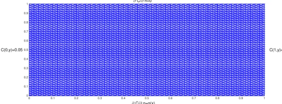
defined over the domain Ω = [0,1]×[0,1], with the parameters u = v = 0.1,
A(y) = 1+e−10y and the boundary conditionsC(0, y) =C(1, y) = 0.05, ∂C∂n = 0 in [0,1]× {1} and ∂C
∂n =g(x) in [0,1]× {0}, where
g(x) = (
0.5 38 ≤x≤ 58,
0 otherwise.
0 0.1 0.2 0.3 0.4 0.5 0.6 0.7 0.8 0.9 1 0
0.1 0.2 0.3 0.4 0.5 0.6 0.7 0.8 0.9 1
C(0,y)=0.05 C(1,y)=0.05
∂ C/∂ n=g(x)
∂ C/∂ n=0
Figure 1: Mesh used in the computation of the numerical solution to (1), along with the boundary conditions for the problem.
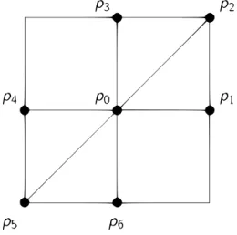
In this mesh, each inner node has six neighbors, as shown in Figure 2. The goal is to find coefficients Γ0,Γ1, ...,Γk such that the following consistency
condition is fulfilled. Consider the second order linear operator:
L(ϕ, K1(x, y), K2(x, y), K3(x, y), K4(x, y), K5(x, y)) =
K1(x, y) ∂2
ϕ
∂x2 +K2(x, y) ∂2
ϕ
∂y2 +K3(x, y) ∂ϕ
∂x +K4(x, y) ∂ϕ
∂y +K5(x, y)ϕ.
This operator evaluated at the grid pointp0 = (x0, y0) leads to the
combi-nation
L0:= 6
X
l=1
Γl(p0, pl, K1(x0, y0), K2(x0, y0),
K3(x0, y0), K4(x0, y0), K5(x0, y0))C(pl),
which must satisfy the consistency condition
τ(p0) := [L(C, K1(x, y), K2(x, y), K3(x, y), K4(x, y), K5(x, y))](x0,y0)−L0→0,
as p1, ...p6 →p0, according to [2].
For the sake of brevity, let
Figure 2: Neighbors distribution for an inner node in the mesh (1).
Let ∆xl and ∆yl be thex and y components ofpl−p0, respectively.
Thus, the local truncation errorτ(p0) (up to second order) yields
τ(p0) = K5(x0, y0)− 6
X
i=0
Γi
!
C(p0) + K3(x0, y0)− 6
X
i=1
Γi∆xi
!
∂C ∂x(p0)
+ K4(x0, y0)− 6
X
i=1
Γi∆yi
!
∂C ∂y(p0)
+ K1(x0, y0)− 6
X
i=1
Γi(∆xi)2
2 !
∂2C ∂x2(p0)
+ −
6
X
i=1
Γi∆xi∆yi
!
∂2C ∂x∂y(p0)
+ K2(x0, y0)− 6
X
i=1
Γi(∆yi)2
2 !
∂2C ∂y2(p0)
+O(max{∆xi,∆yi})3.
If the function C from (1) isCk fork≥2 1, the previous equations can be
1
written as a system of linear equations
1 1 . . . 1
0 ∆x1 . . . ∆x6
0 ∆y1 . . . ∆y6
0 (∆x1)2 . . . (∆x6)2
0 ∆x1∆y1 . . . ∆x6∆y6
0 (∆y1)2 . . . (∆y6)2
Γ0 Γ1 Γ2 . . . Γ6 =
K5(x0, y0) K3(x0, y0)
K4(x0, y0)
2K1(x0, y0)
0 2K2(x0, y0)
. (2)
It is worth to remark that this system of linear equations is not well-determined in general. In order to solve the system (2), the column of zeros and the row of ones can be put aside for a moment to solve the remaining system, and Γ0 can be determined by the first equation of (2)
6
X
i=0
Γi =K5(x0, y0).
Adapting this system to problem (1), the remaining system can be written as
MΓ =β, (3)
according to the node distribution shown in Figure 2, from which it is clear that ∆x = ∆y:= ∆:
M =
∆ ∆ 0 −∆ −∆ 0
0 ∆ ∆ 0 −∆ −∆
∆2 ∆2 0 ∆2 ∆2 0
0 ∆2 0 0 ∆2 0
0 ∆2 ∆2 0 ∆2 ∆2
, Γ = Γ1 Γ2 . . . Γ6
, β=
−u(x0, y0) ∂A
∂y(x0, y0)−v(x0, y0)
2A(x0, y0)
0 2A(x0, y0)
.
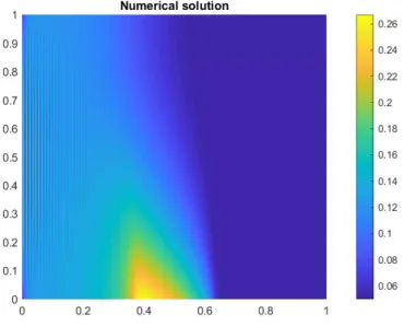
Figure 3: Numerical solution obtained for the problem (1).
3. The inverse problem
In the context of this work, byinverse problem it will be referred the following issue: given the numerical solution obtained for problem (1) in the previous section, suppose that such solution corresponds to an actual measurement of the concentration of a substance suspended in the atmosphere. The inverse problem discussed in this work is about determine some of the physical parameters involved in this advection-diffusion problem starting from the already-known solution; particularly, it will be about determine the parameters u and v from (1), which corresponds to the transport velocities. For the model of these parameters, Dilley and Yen [3] proposed the following functions, given as power laws:
u(x, y) = (U1−ax)
y y1
m
, v(y) = ay
m+ 1
y y1
m
,
where U1, a, y1, m are parameters to be determined, which are closely related
to the physics involved in the problem.
A1 413.86 A2 41.38 B1 0.03 B2 0.03 α1 413.86 α2 0.03
Table 1: Values found for the parameters in (4).
to be less complex that the ones proposed in [3]. The fist approach proposed is given by the following power laws:
u(x) =A1xα1 +B1, v(y) =A2yα2 +B2, (4)
where the coefficients A1, A2, B1, B2, α1, α2 are constants to be determined. In comparison with the models proposed in [3], each of these approaches depends only of one space component, x and y respectively. The calculation of the parameters was made using the data from the numerical solution obtained in the previous section in a non-linear, regularized least-squares adjustment using the trust-region-reflective algorithm. The values found for such parameters are shown in Table 1.
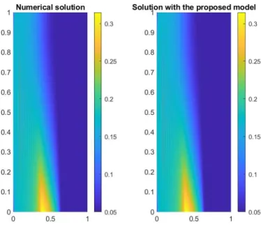
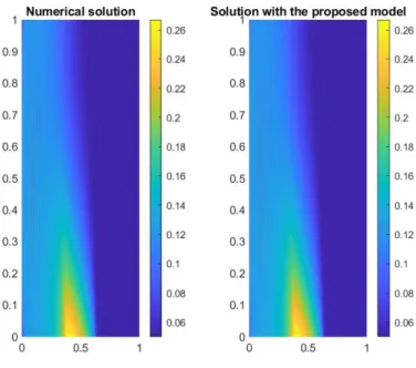
The functions proposed in (4), along with the parameters just found, were used to compute a numerical solution to the problem (1) using the scheme in generalized finite-differences described in the previous section. Both numerical solutions are compared below.
As it can be seen in Figure 4, both numerical solutions are quite similar, which can be confirmed by the norm of the difference between these two matri-ces. The || · ||∞-norm of this difference is 1.608×10⁻¹⁰, while the || · ||2-norm
of this difference is 4.6×10⁻⁹.
The second model proposed is given as rational functions as follows:
u(x) = A1x+A2
A3x+A4, v(y) =
B1y+B2
B3y+B4, (5)
where the coefficientsA1, A2, A3, A4 andB1, B2, B3, B4 are constants to be
de-termined. Just like the model (4), each of these functions depends only on one space coordinate, x and y respectively. Here again, a non-linear, regular-ized least-squares adjustment using the data from the solution obtained in the previous section was used to determine the parameters required. The trust-region-reflective algorithm was also used. The values found for each parameter are shown below:
The numerical solution to (1) was calculated again replacing the functions
Figure 4: Comparison of both numerical solutions, using the expo-nential model (4).
scheme described in the previous section. The comparison between both nu-merical solutions is shown below. For comparison purposes, the norm of the difference between these two matrices was computed again. The || · ||∞-norm
of this difference is 6.57×10⁻¹¹, while the || · ||
2-norm of this difference is
3.21×10⁻⁹.
4. Conclusions
A1 0.0499 B1 0.0501 A2 0.0499 B2 0.0501 A3 0.0501 B3 0.0499
A4 0.0501 B4 0.0499
Table 2: Values found for the parameters in (5).
Regarding section three, we would like to remark that it is possible to model the transport velocities involved in the formulation of problem (1) in a simpler way that the one presented in [3]. It must be recognized that the formulation made in [3] is much more related to the physics involved in the problem, but our claim is that a simpler approach for such parameters is also possible, which is a quite desirable feature when computing a numerical solution.
References
[1] M. Agarwal, A. Tandon. Modeling of the urban heat island in the form of mesoscale wind and of its effect on air pollution dispersal,Applied Mathe-matical Modeling,34(2010), 2520-2530.
[2] M. Celia, W. Gray, Numerical Methods for Differential Equations, Prentice-Hall (1992).
[3] J.F. Dilley, K.T. Yen, Effect of a mesoscale type wind on the pollutant distribution from a line source,Atmos. Environ,6 (1971), 843-851. [4] F.-J. Dom´ınguez-Mota, S. Mendoza-Armenta, J.-G. Tinoco-Ruiz, G.
Tinoco-Guerrero, Numerical solution of Poisson-like equations with Robin boundary conditions using a finite difference scheme defined by an opti-mality condition, In: MASCOT11 Proceedings, IMACS (2011), 101-110.
[5] H.W. Engl,Inverse Problems, Sociedad Matem´atica Mexicana (1995).
[6] J.S. Lin, L.M. Hieldemann, Analytical solution of the atmospheric diffusion equation with multiple sources and height dependent wind speed and eddy diffusivities, Atmos. Environ., 30(1996), 239-254.
Figure 5: Comparison of both numerical solutions, using the rational model (5).
[8] J.J.B. Mu˜noz, F. Ure˜na-Prieto, L.A.G. Corvinos, Solving parabolic and hy-perbolic equations by the generalized finite difference method,J. of Com-put. and Appl. Math., 209, No 2 (2007), 208-233.
[9] J.J.B. Mu˜noz, F. Ure˜na-Prieto, L.A.G. Corvinos, Application of the gen-eralized finite difference method to solve the advection diffusion equation, J. of Comput. and Appl. Math.,2011 (2011), 1849-1855.
[10] G. Tinoco-Guerrero, F.J. Dom´ınguez-Mota, A. Gaona-Arias, M.L. Ruiz-Zavala, J.G. Tinoco-Ruiz, A stability analysis for a generalized finite-difference scheme applied to the pure advection equation, Mathematics and Computers in Simulation,147 (2018), 293-300.