HOW AN ERA OF KINATION IN THE EARLY UNIVERSE IMPACTS DARK MATTER ANNIHILATION SIGNATURES
Kayla Jaye Redmond
A dissertation submitted to the faculty at the University of North Carolina at Chapel Hill in partial fulfillment of the requirements for the degree of Doctor of Philosophy in the Department
of Physics.
Chapel Hill 2019
ABSTRACT
Kayla Jaye Redmond: How an Era of Kination in the Early Universe Impacts Dark Matter Annihilation Signatures
(Under the direction of Adrienne Erickcek)
TABLE OF CONTENTS
LIST OF FIGURES . . . v
LIST OF ABBREVIATIONS AND SYMBOLS . . . vi
INTRODUCTION . . . 1
CHAPTER 1: New Constraints on Dark Matter Production during Kination . . . .9
1.1 Kinaton Cosmology . . . 9
1.1.1 Freeze-Out . . . 12
1.1.2 Freeze-In . . . 16
1.2 Constraints on Kination . . . 21
CHAPTER 2: Growth of Dark Matter Perturbations during Kination . . . 27
2.1 Derivation of the Perturbation Equations . . . 27
2.2 Initial Conditions . . . 30
2.3 Perturbation Evolution . . . 33
2.4 Analytic Expressions . . . 34
2.4.1 Φ Evolution . . . 34
2.4.2 δχ Evolution . . . 37
2.5 The Matter Power Spectrum . . . 42
CHAPTER 3: The Effects of Dark Matter Perturbation Growth during Kination . . . 46
3.1 Dark Matter Transfer Function . . . 46
3.2 Kinetic Decoupling and Free Streaming . . . 50
3.3 Primordial Structures . . . 54
3.4 Boost Factor . . . 58
CHAPTER 4: The Implications of Substructure Boost on Kination Constraints . . . 64
CONCLUSION . . . .73
LIST OF FIGURES
Figure 1.1 Density Evolution of the Kinaton, Radiation, and Dark Matter . . . 11
Figure 1.2 Evolution ofY and Yeq for Freeze-Out Scenario . . . 13
Figure 1.3 Dark Matter Abundance as a Function of hσvi . . . 16
Figure 1.4 Evolution ofdY /da for Freeze-In Scenario . . . 18
Figure 1.5 Allowed Freeze-In Parameter Space formχ andhσvis . . . 22
Figure 1.6 Allowed Freeze-Out Parameter Space formχ and hσvi . . . 22
Figure 1.7 Constraints onmχ and TKR for Freeze-Out Scenarios . . . 24
Figure 2.1 Evolution ofδχ for Modes that Enter Horizon During Kination . . . 34
Figure 2.2 Evolution of Φ for Multiple Cosmologies . . . 36
Figure 2.3 Evolution of Φ for Modes that Enter Horizon During Kination . . . 37
Figure 2.4 Analytical Evolution ofδχ for Modes that Enter Horizon During Kination . . . 39
Figure 2.5 δχ Evaluated for Variousk Modes . . . 43
Figure 3.1 Matter Transfer Function . . . 50
Figure 3.2 Kinetic Decoupling and Free Streaming Scales . . . 53
Figure 3.3 σ(M) with no Cutoff to the Matter Power Spectrum . . . 55
Figure 3.4 σ(M) with Cutoffs to the Matter Power Spectrum . . . 56
Figure 3.5 Evolution ofdf /dlnM . . . 57
Figure 3.6 Evolution of Total Bound Fraction . . . 58
Figure 3.7 Boost Factor . . . 62
Figure 4.1 Constraints onmχ and TKR for Freeze-Out Scenarios with Inverted Axes . . . . 65
Figure 4.2 Minimum Boost Required to Rule Out Freeze-Out Scenarios . . . 67
Figure 4.3 Constraints onMmin . . . 68
Figure 4.4 Constraints onkcut/kKR . . . 70
LIST OF ABBREVIATIONS AND SYMBOLS
a Scale factor
B(M) Boost factor
BBN Big Bang Nucleosynthesis
c Speed of Light
D(a) Growth Function
D(a) Growing solution to Meszaros Equation
δc Critical linear overdensity
δi Fractional density perturbation forith fluid
δρ Dominant fluid’s energy density perturbation
δP Dominant fluid’s pressure perturbation hEχi Average energy of a dark matter particle
f Fraction of dark matter consisting of a thermal relic
fb Baryon fraction
fs Current fraction of dark matter not bound into kination-generated microhalos
ftot Fraction of dark matter bound in halos with M smaller than MKR
F(kR) Filter function
G Gravitational constant GeV Giga Electronvolt
gχ Internal degrees of freedom
g∗(T) Number of relativistic degrees of freedom at temperatureT g∗s(T) Effective number of degrees of freedom at temperature T
H Hubble Parameter
H0 Present-day Hubble Parameter
~ Reduced Planck constant
H.E.S.S. High Energy Stereoscopic System
Jb Bessel function of the first kind
kB Boltzmann constant
λfs Dark matter free streaming length
MeV Mega Electronvolt
mpl Planck mass
mχ Dark matter mass
M⊕ Earth mass
M Solar mass
n Comoving number density of halos
nχ Dark matter number density
nrel Number density of relativistic particles
ns Scalar spectral index
θi Velocity perturbation for ith fluid
σel Dark matter scattering cross section
σ(M) Root-mean-square density perturbation
hσvi Velocity-averaged dark matter annihilation cross section
hσvis s-wave dark matter annihilation cross section for massive particles Ωχh2 Dark matter relic density
Ωdmh2 Dark matter relic density where dark matter is solely a thermal relic ΩM Current matter density divided by current critical density
p Fluid pressure
Pδ Power spectrum of density perturbations
PΦ Power spectrum of curvature fluctuations
ρI Total energy density ata=aI
ρφ Scalar field energy density
ρr Radiation energy density
ρχ Dark matter energy density QCD Quantum chromodynamics
s Entropy density
~s Comoving displacement of massive particles
T Temperature of thermal bath
T(k) Transfer function
Tµν Energy momentum tensor
τ Conformal time
uµ Fluid’s four-velocity
vj Fluid’s comoving peculiar velocity
w Equation of state parameter
x mχ/TF
χ Dark matter particle ¯
χ Dark matter anti-particle Γ(x) Gamma function
Γann Dark matter annihilation rate
Γel Dark matter momentum exchange rate
Y Dimensionless comoving dark matter number density
Yeq Dimensionless comoving dark matter number density in thermal equilibrium
Yb Bessel function of the second kind
z Redshift
Φ Metric perturbation
Φp Superhorizon gravitational potential during radiation domination Φ0 Superhorizon gravitational potential during an era of kination
Ψ Metric perturbation
INTRODUCTION
Dark matter has been an ever evolving area of research spanning back to when Fritz Zwicky coined the term “dark matter” in 1933. Zwicky measuring the radial velocities of galaxies within the Coma cluster, and using the virial theorem, deduced the existence of non-luminous matter within the cluster [1]. Zwicky calculated that the velocities of the galaxies within the Coma cluster were significantly higher than expected, which could only be achieved if there was a non-luminous matter component in the cluster that was subsequently increasing the gravitational force on the galaxies. Observations of M31 by Vera Rubin in 1970 further substantiated Zwicky’s claim of the existence of non-luminous dark matter when it was shown that M31 exhibited a flat rotation curve. Newtonian dynamics predict that the velocities of stars and gas orbiting the center of a galaxy should decrease as the distance from the galactic center extends past the luminous portion of the galaxy. Yet observations of spiral galaxies show that orbital velocities increase and become constant at high distances from the galactic center, thereby producing flat rotation curves. The flat rotation curves are a consequence of dark matter halos encompassing the galaxies [2]. More recently, through an extensive analysis of individual galaxies behind galaxy clusters, the Sloan Digital Sky Survey [3] has also found evidence of dark matter halos using weak gravitational lensing.
Observations of the Cosmic Microwave Background (CMB) from the Wilkerson Microwave Anisotropy Probe (WMAP) [4] and Planck [5] have determined that while roughly 24% of the Universe is composed of dark matter, only 4% of the Universe is made up of baryonic matter. We define baryonic matter as all “ordinary” matter, namely protons, neutrons, and electrons. 1 The CMB power spectrum provides a wealth of information on various cosmological parameters. The total matter density in the Universe is measured primarily from the amplitude of the CMB power spectrum. The CMB also captures the acoustic oscillations inherent in the primordial plasma, from which the baryon density is derived. Before recombination, the baryons and photons are coupled in a plasma. The dark matter is not coupled to the plasma because it is electrically neutral. In the 1
presence of an overdense region, the dark matter and the baryon-photon plasma will infall due to gravity. The dark matter will remain in the overdense region, but the increased photon pressure will cause the baryon-photon plasma to rebound out of the overdense region. Once the photon pressure subsides, the plasma is pulled back in, resulting in an oscillatory motion. This motion is imprinted on the CMB in the relative heights of the first and second peaks, and from this it is determined that 24% of the Universe is dark matter and 4% is baryonic matter. In addition, the abundances of hydrogen and deuterium predicted from Big Bang Nucleosynthesis (BBN) also suggest that only 4% of the Universe is composed of baryonic matter [6, 7]. Therefore, the majority of matter content in the Universe must be composed of non-baryonic dark matter.
The existence of non-baryonic dark matter implies the need for a dark matter production mechanism in the early Universe. In the early Universe, the radiation bath would have been energetic enough to very effectively pair produce dark matter provided that kBT > mχc2, where radiation refers to all relativistic particles,T is the temperature of the radiation bath, andmχis the dark matter mass. If dark matter interacts solely via the weak force, then dark matter cannot be pair produced from photons, nor can dark matter directly annihilate into photons. Therefore, dark matter is pair produced by other relativistic particles, with relativistic leptons or quarks being the most common pair production mechanism. In addition, the thermal production would produce both dark matter and anti-dark matter. Thus, the dark matter would also self-annihilate and produce high-energy particles, which then generate high-energy gamma rays as they scatter or decay into lighter particles.
Observations of dark matter-rich environments look for dark matter annihilation signatures, which are expected to be in the form of gamma rays. For example, there have been observations of dwarf spheroidal galaxies by the Fermi Gamma-Ray Telescope [8] and observations of the Galac-tic center by the High Energy Stereoscopic System (H.E.S.S.) [9]. The absence of dark matter annihilation signatures has placed tight constraints on the dark matter mass and the dark mat-ter annihilation cross section. These constraints have ruled out scenarios where dark matmat-ter is thermally produced during radiation domination for all dark matter masses below 120 GeV.
enough, such that the rate of dark matter pair production equals the rate of dark matter an-nihilations. As the radiation bath cools pair production stops, but dark matter annihilations continue, thereby reducing the dark matter abundance. The dark matter deviates from ther-mal equilibrium and “freezes out” when the Hubble expansion rate H equals the dark matter annihilation rate Γann and the average time between annihilations becomes longer than the age
of the Universe. Therefore, the temperature at which freeze-out occurs TF, is defined as when
H(TF) = Γann(TF) =nχ(TF)hσvi, where nχ(TF) is the dark matter number density at freeze-out.
If dark matter freezes out during radiation domination, nearly all dark matter annihilations cease at freeze-out. Therefore, rescaling the dark matter density from freeze-out to today allows us to calculate the current dark matter relic abundance Ωχh2. For dark matter that freezes-out during radiation domination, Ωχh2 ∝(mχ/TF)(1/hσvi) andmχ/TF∼20. Therefore, the dark matter relic
abundance is largely independent of the dark matter mass and to obtain the observed dark matter relic abundance Ωχh2 = 0.12 [5] requires hσvi= 3×10⁻²⁶cm3/s [14]. This calculation of hσvi is referred to as the WIMP miracle because it matches, to within a factor of 10, the annihilation cross section predicted for 100 GeV dark matter particles annihilating via the weak force. Unfortunately, supersymmetric (SUSY) models find it difficult to obtain scenarios with hσvi= 3×10⁻²⁶cm3/s [15]. For example, Binos naturally want hσvi<3×10⁻²⁶cm3/s and Winos and Higgsinos nat-urally want hσvi>3×10⁻²⁶cm3/s [15]. However, the requirement that hσvi= 3×10⁻²⁶cm3/s assumes that the early Universe is solely radiation dominated. If we assume a different thermal history, in which something other than radiation dominates the energy density of the Universe prior to BBN, then to obtain the observed dark matter relic abundance may require hσvi values that deviate from 3×10⁻²⁶cm3/s, thereby allowing more generic SUSY models to become viable dark matter candidates [16, 17].
In the simplest model, inflation is powered by a scalar field defined as the inflaton, and the Universe becomes radiation dominated when the inflaton decays into relativistic particles shortly after the end of inflation [26, 27, 28]. An alternative scenario is that a fast-rolling scalar field (a kinaton) dominates the energy density of the Universe prior to the onset of radiation domination. When the kinaton’s energy density is dominant, the Universe is said to be in a period of kination [29, 30, 31]. Kination was initially proposed as an inflationary model that does not require the complete conversion of the inflaton energy into radiation to initiate the onset of radiation domination [29]. Kination also facilitates baryogenesis; if the electroweak phase transition occurs during kination, then baryogenesis is possible during a second-order phase transition [30]. Finally, if the kinaton’s potential energy becomes dominant at very late times, it can accelerate the expansion of the Universe and mimic the effects of a cosmological constant [31, 32, 33, 34, 35].
The uncertainties in the thermal history of the Universe prior to BBN limit our understanding of the origins of dark matter [17, 36, 37, 38, 39, 40, 41, 42, 43]. We study the effects of kination on the thermal production of dark matter. We derive analytic expressions for the dark matter relic abundance generated during kination and confirm that our analytic results match the numeric solutions to the Boltzmann equation. Our relic abundance expressions depend on the dark matter massmχ, the velocity-averaged dark matter annihilation cross sectionhσvi, and the temperature at which the Universe becomes radiation dominated,TKR. Our analytic expressions allow us to solve
on mχ and hσvi from Fermi-LAT PASS-8 observations of dwarf spheroidal galaxies [8] and High Energy Stereoscopic System (H.E.S.S.) observations of the Galactic center [9], we constrain TKR
for scenarios where dark matter freezes out during an era of kination. We determine that kination scenarios in which dark matter freezes out have a minimum allowed value ofTKRbetween 0.05 GeV
and 1 GeV, depending on the dark matter annihilation channel.
We also study what effects an era of kination has on the growth of dark matter density perturba-tions. If dark matter density perturbations experience sufficient growth during an era of kination, this could generate enhanced substructure and increase the dark matter annihilation rate. The annihilation rate for dark matter Γann∝ρ2χ, whereρχis the dark matter energy density. The pres-ence of substructure increasesρχand therefore increases the dark matter annihilation rate, which is referred to as a substructure boost. The boost factor for a halo quantifies how the annihilation rate differs compared to if the halo has a smooth density profile. If dark matter produced during an era of kination yields boost factors ∼ 10, then we could rule out the equilibrium thermal production of dark matter for the bb,τ+τ−, and W+W− annihilation channels. It has been shown that dark matter produced during an early-matter dominated era (EMDE) yields boost factors ranging from 10−104, and these boost factors were sufficient enough to bring some EMDE scenarios into ten-sion with constraints put forward by Fermi-LAT observations of dwarf spheroidal galaxies [42, 44]. Therefore, it may be possible to achieve the boost factors required to rule out certain kination scenarios.
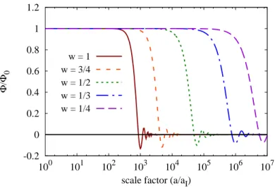
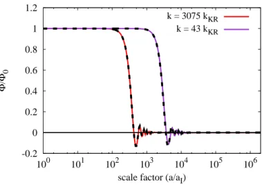
We perform a perturbation analysis given that dark matter is thermally produced during an era of kination to determine what effects this has on structure growth. We derive analytic expressions for the evolution of the gravitational potential Φ and dark matter density perturbationsδχnot only during an era of kination, but also for scenarios where the dominant component of the Universe has a generic equation of state parameter, w. We determine that once a mode enters the horizon, the gravitational potential drops sharply and then oscillates with a decaying amplitude if the dominant energy density hasw >0. In addition, ifw >1/3, thenδχ∝a3w/2−1/2, whereais the scale factor. Therefore, if a perturbation mode enters the horizon during an era of kination (w = 1), then δχ grows linearly with the scale factor. This growth leaves an imprint on the matter power spectrum. We determine that for modes that enter the horizon during an era of kination,δχ/Φ0 ∝k1/2, where
scales during kination.
Our perturbation analysis is applicable for scenarios in which dark matter does and does not reach thermal equilibrium during an era of kination. References [45, 46] determined that if dark matter reaches thermal equilibrium during an era of kination, annihilations do not cease until after the Universe becomes radiation dominated. We determine that these “relentless” annihilations do not significantly influence the evolution of δχ after a mode has entered the horizon. Since dark matter annihilation cannot lead to deviations from adiabaticity on superhorizon scales [47, 48, 49], “relentless” annihilation has a minimal effect on the matter power spectrum.
Due to the fact that dark matter density perturbations experience enhanced growth for modes that enter the horizon during an era of kination, we take our analysis further and study how this influences the dark matter annihilation rate and the corresponding boost factor. The boost factor is determined by the minimum halo mass, which is determined by the cutoff to the matter power spectrum. The cutoff to the matter power spectrum suppresses power for modes withk > kcut and
is determined by the temperature at kinetic decoupling. The kinetic decoupling of dark matter occurs when the dark matter ceases to efficiently exchange momentum with relativistic particles. The momentum exchange rate for non-relativistic dark matter scattering off of relativistic particles is Γel. Once Γel =H, the dark matter kinetically decouples from the relativistic particles and the
average time between collisions becomes longer than the age of the Universe. The kinetic decoupling temperature Tkd is defined from the relation Γel(Tkd) =H(Tkd) and the wavenumber of the mode
that enters the horizon at kinetic decoupling is kkd. We assume that kinetic decoupling occurs
against being pulled out of overdense regions and the oscillations to the dark matter perturbations become damped compared to the oscillations to the radiation perturbations. Therefore, the later kinetic decoupling occurs increases the amount of damping on the dark matter density perturbations and influences the cutoff to the matter power spectrum.
Kinetic decoupling also sets the dark matter free-streaming length, λfs. The free-streaming
length is the distance covered by the dark matter from the time of kinetic decoupling to the present. Dark matter perturbations with wavelengths less than λfs ≡k−fs1 will be washed out and
not participate in structure growth [50]. To account for both the effects of kinetic decoupling and free-streaming, perturbations with k > kcut are suppressed, with kcut being the smaller of kkd
and kfs [50]. The cutoff scale not only sets the mass of the smallest halos, it also determines the
substructure boost.
We determine that the boost factors produced from structure growth during an era of kination are insufficient to constrain freeze-in scenarios. On the other hand, we are able to further constrain scenarios where freeze-out occurs during an era of kination. For each of the allowed freeze-out parameter sets, we calculate the minimum boost required to rule out each scenario based on obser-vational bounds from dwarf spheroidal galaxies. Obserobser-vational bounds set by the Galactic center are not considered when determining the minimum boost because we assume that all microhalos near the Galactic center are destroyed by tidal stripping or stellar encounters, and thus there is no substructure boost. From the minimum boost required to rule out each kination scenario, we work backwards and calculate the maximum allowed value of Tkd/TF. For the parameter space we are
looking to constrain, the maximum allowed value for Tkd/TF ranges from 10−2 to 104.
Over the scope of this research, we have placed constraints on mχ,TKR, and hσvifor scenarios
where dark matter freezes out during an era of kination. We have calculated how perturbations evolve for modes that enter the horizon during an era of kination. Upon learning that perturbations experience enhanced growth during an era of kination, we calculated the boost factors resulting from the amplified structure growth. While we could not constrain the freeze-in scenarios, we were able to place further constraints on the freeze-out scenarios. Specifically, we placed additional constraints on the maximum allowed values ofTkd/TF.
use observational data from Fermi-LAT and H.E.S.S. to constrainmχ,TKR, andhσvi. In Chapter
2, we present the evolution equations that govern density and velocity perturbations. We also derive analytic expressions for the evolution of the gravitational potential and dark matter density perturbations and determine how the matter power spectrum scales with wavenumber following an era of kination. In Chapter 3, we derive the dark matter transfer function, taking into account an era of kination. We also detail how kinetic decoupling and free-streaming influence the matter power spectrum and growth of primordial structures. Finally, we derive the substructure boost and compare the boost from structure growth during an era of kination to that during radiation domination. In Chapter 4, we present updated constraints on the remaining allowed kination scenarios by determining the maximum allowed values ofTkd/TF. In the conclusion, we summarize
CHAPTER 1: New Constraints on Dark Matter Production during Kination
1.1 Kinaton Cosmology
The scenario we consider consists of a fast-rolling scalar field (the kinaton) that dominates the energy density of the Universe prior to BBN. The kinaton’s energy density is dominated by its kinetic energy, meaning that the kinaton’s energy density equals its pressure and that the equation of state parameter is w = 1. Therefore, the kinaton’s energy density scales as a−6, where a is the scale factor, and will eventually become subdominant to radiation, whose energy density scales as a−4. Kinaton-radiation equality is defined as the point at which the radiation energy density becomes the dominant component of the Universe. It is important to note, however, that during kination, the temperature of the radiation bath is higher than the temperature at kinaton-radiation equality. Therefore, it is possible to thermally produce dark matter prior to the onset of radiation domination.
We consider three energy density components during kination: dark matter, radiation, and the kinaton. The evolution of these energy densities are governed by three free parameters: the dark matter mass mχ, the temperature at kinaton-radiation equality TKR, and the velocity-averaged
dark matter annihilation cross sectionhσvi. Throughout this work, we assumes-wave dark matter annihilation. In kination scenarios, TKR is the temperature at which the radiation energy density
equals the kinaton energy density. We assume that the kinaton does not decay nor interact with dark matter or radiation (see Ref. [51] for an analysis of decaying kinaton cosmologies). Radiation and dark matter on the other hand are thermally coupled via pair production and annihilation. Therefore, the equations for the energy density of the scalar field ρφ, the radiation energy density
The content of this chapter has been published as an article in Physical Review D. The original citation is as follows: Kayla Redmond and Adrienne L. Erickcek. New Constraints on Dark Matter Production during Kination. Phys.
ρr, and the dark matter number density nχ are
d
dtρφ=−6Hρφ, (1.1a)
d
dtnχ=−3Hnχ− hσvi(n
2
χ−n2χ,eq), (1.1b)
d
dtρr =−4Hρr+hσviEχ(n
2
χ−n2χ,eq), (1.1c)
wherehEχi=ρχ/nχis the average energy of a dark matter particle andnχ,eq is the number density
of dark matter particles in thermal equilibrium.2 For a dark matter particle with mass mχ and internal degrees of freedom gχ within a thermal bath of temperatureT,
nχ,eq =
gχ 2π2
Z ∞
mχ q
E2−m2
χ
eE/T + 1 EdE. (1.2)
When evaluating the average energy of a dark matter particle, we make the approximation that hEχi '
q m2
χ+ (3.151T)2, which matchesρχ/nχ to within 10%.
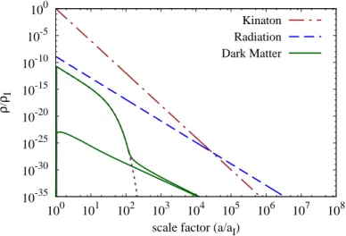
Figure 1.1 shows the evolution of the kinaton, radiation, and dark matter densities obtained by numerically solving Eq. (1.1). Initially, the kinaton’s energy density is dominant, but since it scales away more quickly than the radiation energy density, it eventually becomes subdominant. Figure 1.1 shows that the radiation energy density scales asa−4 and is unaffected by dark matter annihilation or pair production. Since ρr and ρφevolve independently ofnχ, we can solve for their evolution analytically. We then use these solutions to numerically solve Eq. (1.1b) and calculate the dark matter relic abundance.
To accurately describe the evolution ofρr, we need to take into account the energy injection that occurs when Standard Model particles become nonrelativistic. When a particle species becomes nonrelativistic, its entropy is transferred to the remaining relativistic particles. Entropy is conserved during kination; therefore, the universal entropy sa3 must remain constant, where sis the entropy density: s≡(2π2/45)T3g∗s(T), and g∗s(T) is the effective number of degrees of freedom that
contribute to the entropy density. Due to the conservation of entropy, radiation cools during kination according to the same proportionality as during radiation domination: T ∝g∗s(T)−1/3a−1. To evaluate the temperature of the radiation bath, we set a maximum temperature of TMAX
2
10-35 10-30 10-25 10-20 10-15 10-10 10-5 100
100 101 102 103 104 105 106 107 108
ρ
/
ρI
scale factor (a/aI) Kinaton Radiation Dark Matter
Figure 1.1: The density evolution of the kinaton, radiation, and dark matter. In this figure,
mχ = 104GeV, and kinaton-radiation equality occurs when a/aI = 2.7×10⁴; the temperature at kinaton-radiation equality is 2 GeV. The two solid curves show the evolution of ρχ for the two values ofhσvithat produce the observed dark matter density: Ωχh2= 0.12 [5]. The top solid curve corresponds to the freeze-out scenario with hσvi= 7.5×10⁻²⁵cm3s−1, whereas the bottom solid
curve corresponds to the freeze-in scenario withhσvi= 6.7×10−46cm3s−1. The dotted line shows the equilibrium dark matter density,ρχ,eq =hEχinχ,eq.
at which ρχ = 0. We set TMAX= 8mχ to ensure that if the dark matter is capable of reaching thermal equilibrium, it will have adequate time to do so. If the dark matter cannot reach thermal equilibrium, setting TMAX= 8mχ ensures there will be enough time for maximal pair production. Therefore, the dark matter relic abundance will not be sensitive toTMAX. UsingTMAX, we construct
an expression for the temperature evolution during kination that accounts for changes ing∗s(T):
T =TMAX
g∗s(TMAX)
g∗s(T)
1/3 aI
a, (1.3)
whereaI is the scale factor value whenT =TMAX.
The final step in evaluating ρr is to connect Eq. (1.3) and the definition of ρr. The radiation energy density isρr≡(π2/30)g∗(T)T4, whereg∗(T) is the number of relativistic degrees of freedom
at temperatureT. Using this definition of ρr and Eq. (1.3), we see that the evolution of ρr during kination is
ρr=
π2
30 g∗(T)T
4 MAX
g∗s(TMAX)
g∗s(T) 4/3
aI a
4
Next, we analytically solve for ρφ. Solving Eq. (1.1a) yields ρφ=ρφ,I(aI/a)6, where ρφ,I is ρφ when a= aI. By defining aKR as the scale factor value at the onset of radiation domination we
see thatρφevaluated at kinaton-radiation equality equals ρφ,I(aI/aKR)6. Using Eq. (1.4), we can
evaluateρr at kinaton-radiation equality. Considering that at kinaton-radiation equality ρφ=ρr, this implies that
ρφ,I =
π2
30g∗(TKR)T
4 MAX
g∗s(TMAX)
g∗s(TKR)
4/3 aKR
aI
2
. (1.5)
Using Eq. (1.3) to relateaKR toTKR, we obtain the evolution of ρφ during kination:
ρφ=
π2
30
TMAX3
TKR 2
g∗s(TMAX)
g∗s(TKR) 2
g∗(TKR) aI
a 6
. (1.6)
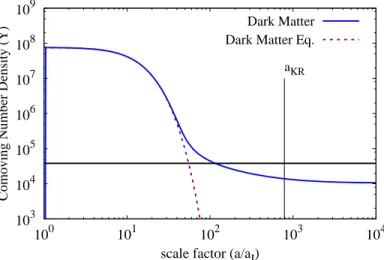
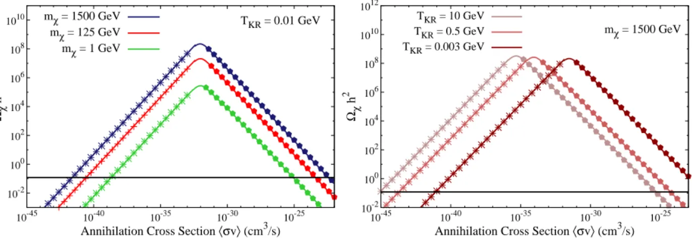
Now that we have obtained expressions for T(a), ρr(a) and ρφ(a), we have the necessary com-ponents to numerically solve Eq. (1.1b) for nχ(a), as shown in Figure 1.2. Figure 1.3 shows the dark matter relic abundance as a function of hσvi for several values of TKR and mχ. For small hσvi values, the dark matter cannot reach thermal equilibrium, and Figure 1.3 shows that ashσvi increases the dark matter relic abundance increases. Oncehσvibecomes large enough, pair produc-tion will bring nχ up to its thermal equilibrium value. If dark matter reaches thermal equilibrium, we see from Figure 1.3 that as hσvi increases, the dark matter relic abundance decreases. In the following sections, we derive analytic expressions for the dark matter relic abundance generated during kination and analyze how the relic abundance is influenced byTKR.
1.1.1 Freeze-Out
If hσvi is sufficiently large, then pair production brings dark matter into thermal equilibrium:
nχ=nχ,eq, as defined in Eq. (1.2). OnceH' hσvinχ,eq, the dark matter deviates from equilibrium
and “freezes out”. If dark matter freezes out during radiation domination, nearly all dark matter annihilations cease at freeze-out. However, if dark matter freezes out during kination, we see from Figure 1.2 that we need to take dark matter annihilations between the time of freeze-out and kinaton-radiation equality into account to get an accurate relic abundance.
103 104 105 106 107 108 109
100 101 102 103 104
Comoving Number Density (Y)
scale factor (a/aI)
Dark Matter Dark Matter Eq.
aKR
Figure 1.2: The evolution of the comoving dark matter number density and equilibrium number density with TKR= 20 GeV, mχ= 3000 GeV, and hσvi= 10−32cm3s−1. The vertical line repre-sents the point of kinaton-radiation equality at aKR/aI = 800. The solid horizontal line shows the comoving number density at the point of freeze-out solved from H(TF) =hσvinχ,eq. This figure
demonstrates that dark matter annihilations after freeze-out significantly decrease the dark matter number density.
Equation (1.1b) is rewritten as
dY
da =hσvi TKR3 a3I
Ha4 (Y 2
eq−Y2). (1.7)
After the dark matter freezes out,Y2 Yeq2. Since during kinationH =H(aI)[aI/a]3, we simplify Eq. (1.7) to
dY
da =
−λKD
a Y
2, (1.8)
where λKD=TKR3 hσvi/H(aI). Integrating Eq. (1.8) from freeze-out to kinaton-radiation equality yields
1
YF
− 1
YKR
=−λKD ln
aKR
aF
, (1.9)
where YF and YKR are the comoving dark matter number densities at freeze-out and
To evaluate the current dark matter density we need to reevaluate Eq. (1.7) during radiation domination and solve forY at some late time. During radiation dominationH=H(aKR)[aKR/a]2,
and by definingλRD= [TKR3 hσvi/H(aKR)]×[a3I/a2KR], Eq. (1.7) simplifies to
dY
da =
−λRD
a2 Y
2. (1.10)
Solving Eq. (1.10) from kinaton-radiation equality to a very late time yields
1
YKR
− 1
YLT
=−λRD
1
aKR
, (1.11)
where YLT is the comoving dark matter number density at some late time (a =aLT). To obtain
Eq. (1.11), we use the fact thataLTaKR. Therefore, if dark matter freezes out during kination,
Y experiences a logarithmic decrease between freeze-out and kinaton-radiation equality, after which
Y approaches a constant value.
Utilizing YKR from Eq. (1.9) and rewriting Eq. (1.11) in terms of the dark matter number
density yields
nχ,LT=
hσvia3 LT
H(aI)a3I
ln aKR aF + 1 + a 3 LT
nχ,F a3F −1
. (1.12)
We wish to express Eq. (1.12) in terms of our free parametersmχ,TKR, and hσvi. We can express
H(aI) andaKRin terms ofTKRandTMAXusing Eqs. (1.3) and (1.5). In addition, sincenχ,F 'nχ,eq,
nχ,F 'H(TF)/hσvi. If freeze-out occurs during kination, H2 '(8πG/3)ρφ; combining this with Eqs. (1.3) and (1.6) allows us to solve forH(TF):
H(TF) =
4π3
45
1/2 TF3 mplTKR
g∗sF
g∗sKR
g∗1/KR2 , (1.13)
whereg∗sKR =g∗s(TKR) andg∗KR=g∗(TKR). These relations allow us to rewrite Eq. (1.12) as
nχ,LT=
4π3
45
1/2
TLT3 g∗sLTg1∗/KR2
hσvimplTKRg∗sKR
ln
" TF
TKR
g∗sF
g∗sKR 1/3#
+ 2
!−1
, (1.14)
roughly between 20 and 30.
After aLT,nχ ∝a−3, which allows us to relate the dark matter density ataLT to today:
ρχ,0 =ρχ,LT
aLT
a0 3
=ρχ,LT
T0
TLT 3
g∗s0
g∗sLT
, (1.15)
where T0 is the radiation temperature today and g∗s0= 3.91. Bringing all of the previous
com-ponents together and scaling our analytic expression by a factor of 1.22, thereby ensuring that it matches the numeric solution of Eq. (1.1b) within 20% for mχ/TKR >100, we obtain an analytic
expression for the freeze-out dark matter relic abundance:
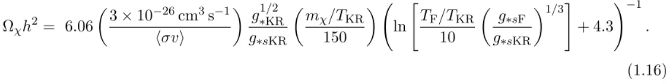
Ωχh2 = 6.06
3×10⁻²⁶cm3s−1
hσvi
g∗1/KR2 g∗sKR
mχ/TKR
150
ln
"
TF/TKR
10
g∗sF
g∗sKR 1/3#
+ 4.3
!−1
.
(1.16)
Equation (1.16) indicates that decreasing TKR increases the relic abundance. Decreasing TKR
re-quires increasing the kinaton energy density, which increases the Hubble parameter during kination. Sincenχ,F 'H(TF)/hσvi, increasing the Hubble parameter increases the dark matter number
den-sity at freeze-out and thus increases the relic abundance. Furthermore, in our calculation of YKR
we showed that dark matter annihilations do not cease during kination. As a result, Eq. (1.16) includes an inverse logarithmic term that depends on the ratioTF/TKR.
Figure 1.3 shows the dark matter relic abundance as a function of hσvi for several values of
TKR and mχ. In Figure 1.3 we see that for sufficiently large hσvi the freeze-out dark matter relic
abundances from Eq. (1.16), represented by the circular symbols, match the numeric solutions to Eq. (1.1b), represented by the curves. We can solve for the minimumhσvithat will result in the dark matter reaching thermal equilibrium. If dark matter freezes out, H(TF) =hσvinχ,eq, and we can
rewrite this equation in terms of a new variablex, wherex≡mχ/TF. Assuming that dark matter is
nonrelativistic, H(TF) =hσvinχ,eq can be rewritten as x−3/2exg∗s(mχ/x) =constant× hσvi. The left-hand side of this equation has a minimum value near x∼1.5 which implies that there is a minimumhσvi for which a solution will exist. This lower bound on hσvi is
hσvi> 9.37×10⁻³³cm3s−1
2 gχ 3 MeV TKR
g∗1/KR2 g∗sKR
!
10-2 100 102 104 106 108 1010
10-45 10-40 10-35 10-30 10-25
Ωχ
h
2
Annihilation Cross Section 〈σv〉 (cm3/s)
mχ = 1500 GeV mχ = 125 GeV mχ = 1 GeV
TKR = 0.01 GeV
10-2 100 102 104 106 108 1010 1012
10-45 10-40 10-35 10-30 10-25
Ωχ
h
2
Annihilation Cross Section 〈σv〉 (cm3/s)
TKR = 10 GeV TKR = 0.5 GeV TKR = 0.003 GeV
mχ = 1500 GeV
Figure 1.3: The observed dark matter abundance Ωχh2 as a function of the dark matter velocity-averaged annihilation cross sectionhσvi. Dark matter freezes in at smallhσviwhere Ωχh2 ∝ hσvi, whereas dark matter freezes out at large hσvi where Ωχh2 ∝ hσvi−1. In the left panel we see
that decreasing mχ decreases Ωχh2 for both cases. In the right panel we see that decreasingTKR
decreases Ωχh2 for the freeze-in case but increases Ωχh2 for the freeze-out case. In both panels the solid curves represent the numerical solutions to Eq. (1.1), while the symbols represent the analytic approximations represented by Eqs. (1.16) and (1.21). The solid black line represents the Planck measurement for the observed dark matter abundance, Ωχh2 = 0.12 [5].
The horizontal line in Figure 1.3 represents the Planck measurement of the observed dark matter abundance. To reproduce the observed dark matter abundance, freeze-out cases during kination require larger hσvi than that required if freeze-out occurs during radiation domination. This comes from the fact that at a given temperature the Hubble parameter during kination is always higher than it is during radiation domination, which causes freeze-out to occur earlier. In order to compensate for the earlier freeze-out and reproduce the observed dark matter abundance, freeze-out scenarios during kination require hσvi>3×10⁻²⁶cm3s−1. Since this lower bound on hσvi is more stringent than Eq. (1.17), Eq. (1.16) is applicable to all freeze-out scenarios that generate the observed dark matter abundance.
1.1.2 Freeze-In
In freeze-in scenarios, the dark matter number density does not reach thermal equilibrium, so nχnχ,eq. The dimensionless comoving dark matter equilibrium number density is Yeq ≡
nχ,eqTKR−3(a/aI)3, and for freeze-in scenarios Yeq Y. Therefore, Eq. (1.7) reduces to
dY
da =
hσviTKR3 H(aI)a
Yeq2 (1.18)
for freeze-in scenarios during kination.
Equation (1.18) implies that dY /da diverges as a→ 0 if hσvi is independent of temperature. The same divergence occurs if the Universe is radiation dominated during dark matter production, and it would make the freeze-in abundance of dark matter dependent onTMAX. Previous analyses of
the freeze-in process avoided this sensitivity to high-energy physics by assuming thathσvi ∝1/ T2
for relativistic particles [52, 53]. We take the same approach and set hσvi=hσvis(mχ/T)2 for
T > mχ and hσvi=hσvis for T < mχ, where hσvis is the s-wave dark matter annihilation cross section for massive particles. With this scaling, dY /da→0 as a→0, and the production of dark matter is finite during kination even if TMAX → ∞. Figure 1.4 shows that dY /da increases until
a=a∗, which we define as the scale factor value at which pair production peaks. The
tempera-ture at which pair production peaks is T∗ = mχ. Therefore, dY /da reaches its maximum when a∗/aI= 8[g∗s(TMAX)/g∗s(T∗)]1/3.
Figure 1.4 also indicates that the integral ofdY /daconverges;Y will approach a constant value as pair production becomes less and less efficient. However, Eq. (1.18) is only valid during kination, so it will only provide an accurate dark matter density if nearly all the pair production occurs prior to kinaton-radiation equality. Truncating the integration ofdY /daataPP, whereT(aPP) =mχ/3.9, reduces the value of Y by less than 1% compared to integratingdY /da out to a=∞. Therefore, pair production has effectively halted whenT < mχ/3.9, and we can use Eq. (1.18) to compute the relic abundance of dark matter provided thatTKR < mχ/3.9. Integrating Eq. (1.18) from 0 toaPP,
while taking into account the fact thathσvichanges from hσvis(mχ/T)2 tohσvis atT =mχ, gives
YPP= 3.1×10⁻⁴
TMAX/TKR
150
3 TKR
5 GeV
gχ
2
2 hσvis
10−45cm3s−1
g∗sKR
g1∗KR/2 !
g∗sMAX
g2 ∗s(mχ)
.
0 20 40 60 80 100
0 5 10 15 20 25 30 35
dY/da
scale factor (a/aI)
a*
Figure 1.4: The evolution of dY /da given TKR = 1 GeV, mχ= 5×10⁴GeV, and hσvis= 10−47cm3s−1. The vertical line represents the scale factor at which pair produc-tion peaks, defined as a∗. For kination scenarios where dark matter freezes in andTMAX = 8mχ,
a∗/aI'8.
After pair production ends,Y remains nearly constant, and thus YPP =YKR. Therefore, the dark
matter density at kinaton-radiation equality can be written as
ρχ,KR =mχYPPTKR3 (aI/aKR)3. (1.20)
Equation (1.3) indicates that (aI/aKR)3 ∝ TMAX−3 g∗−s1MAX. As a result, inserting Eq. (1.19) into
Eq. (1.20) seems to indicate that ρχ,KR is independent of TMAX, but this is not generically true.
When integrating Eq. (1.18) from a = 0 to aPP to obtain Eq. (1.19), we effectively integrated
fromT =∞ toT =mχ/3.9. However, integrating instead fromT = 8mχ toT =mχ/3.9 does not significantly change the result. Therefore, if TMAX≥8mχ, the freeze-in dark matter abundance
does not depend on TMAX. Conversely, if TMAX<8mχ, ρχ,KR will decrease as TMAX decreases
because maximal pair production is not reached.
the freeze-in dark matter relic abundance:
Ωχh2 = 1.08
mχ
1 GeV
TKR
100 GeV
gχ
2
2 hσvis
10−45cm3s−1
g∗sKR
g1∗KR/2 !
g∗−s2(mχ). (1.21)
Equation (1.21) indicates that increasing TKR leads to a larger relic abundance. To understand
how the freeze-in dark matter relic abundance relates toTKR we need to investigate hownχrelates to the Hubble parameter. The connection between the Hubble parameter and nχ stems from the cooling rate dT /dt. During kination T ∝a−1, and therefore dT /dt=−HT. Rewritingdn/dt as a function of temperature yieldsdn/dt= (dT /dt) (dn/dT) =f(T), wheref(T) is the right-hand side of Eq. (1.1b). This allows us to expressdn/dT as
dn
dT =
−f(T)
HT , (1.22)
which implies that n∝1/H. Since increasing TKR decreasesH during kination, it also decreases
the cooling rate, leaving more time for pair production and thereby increasing the dark matter number density.
In order to reach the observed dark matter abundance, scenarios in which dark matter freezes in during kination require largerhσvisvalues than if freeze-in occurs during radiation domination. For example, given a dark matter mass of 100 GeV, a freeze-in scenario during radiation domination requires hσvis= 10−47cm3s−1 in order for Ωχh2= 0.12 [54, 5]. For the same mχ, a freeze-in scenario during kination withTKR = 0.033 GeV requireshσvis= 10−41cm3s−1. Freeze-in scenarios during kination require largerhσvisvalues to generate the observed dark matter abundance because the increased cooling rate during kination leaves less time for pair production.
being nonrelativistic:
Yeq(a) =gχ
a aI
3 TKR−3
mχT
2π 3/2
e−mχ/T. (1.23)
Evaluating Eq. (1.23) at a∗ and equating that to Eq. (1.19) gives us the cross sections that will
result in dark matter freezing in during kination:
hσvis≤ 8.5×10⁻³⁴cm3s−1 g
1/2 ∗KR
g∗sKR !
g∗s(mχ)
2
gχ
3 MeV
TKR
. (1.24)
Figure 1.3 demonstrates that there is a range of hσvis values for each value of TKR where
neither a freeze-out nor freeze-in scenario will result in the observed dark matter abundance. The left panel of Fig. 1.3 shows that, for a fixedTKR, decreasingmχincreases the freeze-in cross section and decreases the freeze-out cross section that generates the observed dark matter abundance. However, oncemχ.3TKR, dark matter will no longer freeze in during kination, and as discussed in
Section 1.1.1,hσvi>3×10⁻²⁶cm3s−1 is required to generate the observed dark matter abundance if dark matter freezes out during kination.
The right panel of Fig. 1.3 shows that decreasingTKR increases the cross section that generates
the observed dark matter abundance via the freeze-in mechanism. Therefore, settingTKR= 3 MeV
gives an upper bound on the cross sections that can generate the observed dark matter abundance in freeze-in scenarios:
hσvis <2.66×10−38cm3s−1
0.175 GeV
mχ
. (1.25)
This maximal cross section is calculated usingg∗s(mχ) =g∗s(0.175 GeV). When deriving Eq. (1.21)
we assumed that g∗s(T) was approximately constant during pair production, which implies that
Ωχh2 ∝g∗−s2(mχ). If dark matter freezes in during kination andmχis less than 0.17 GeV, then the QCD phase transition occurs before the peak of pair production. At the QCD phase transition
The relic abundances from Eq. (1.21) are within 20% of the solutions to Eq. (1.1b) for mχ > 0.17 GeV andTKR < mχ/3.9. If mχ≤0.17 GeV, we need to take into consideration the evolution of g∗s(T) to accurately calculate the relic abundance. Allowing for the evolution ofg∗s(T), YPP is
rewritten as
YPP=
45 4π3
1/2 h
σvismpl
TKR2 g∗1KR/2 TMAX3
m6
χ
g∗sMAXg∗sKR
×
Z 1
0
n2χ,eqx7g∗−s2(mχ/x)dx +
Z xPP
1
nχ,2eqx5g−∗s2(mχ/x)dx
. (1.26)
Using this expression forYPPand a scaling factor of 0.4, we construct a modified relic abundance
ex-pression that takes into account the evolution ofg∗s(T). For freeze-in scenarios withmχ≤0.17 GeV and TKR < mχ/3.9, this updated expression for YPP brings the analytic relic abundance solutions
to within 25% of the numeric solution to Eq. (1.1b).
1.2 Constraints on Kination
To constrain kination cosmologies, we first solve Eqs. (1.16) and (1.21) for all combinations of the variablesmχ,TKR, andhσvi that produce the observed dark matter abundance of Ωχh2 = 0.12 [5]. We set the minimum allowed temperature of kinaton-radiation equality to 3 MeV to ensure that the period of kination does not alter the cosmic microwave background or the abundances of light elements [21, 22, 23, 24, 25].3 Next, we compare our allowed parameters to current constraints on
mχ andhσvifrom Fermi-LAT and H.E.S.S. Specifically, we use the Fermi-LAT PASS-8 constraints from observations of dwarf spheroidals [8] and H.E.S.S. constraints from observations of the Galactic center [9]. The Fermi-LAT data covers dark matter masses ranging from 2 GeV≤mχ≤104GeV, while the H.E.S.S. data covers dark matter masses ranging from 125 GeV≤mχ ≤7×10⁴GeV.
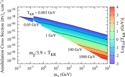
Figure 1.5 shows the allowed parameter space for mχ and hσvis for scenarios in which dark matter freezes in during kination. To ensure that freeze-in occurs before the onset of radiation domination, we have restricted ourselves to mχ/3.9> TKR. This restriction comes from the fact
that the temperature at which pair production effectively ceases is TPP = mχ/3.9. Since the minimum value of TKR is 3 MeV, we require thatmχ>0.012 GeV to ensure that freeze-in occurs 3
These constraints onTKRwere derived assuming that the radiation-dominated era was preceded by an
10-2 10-1 100 101 102 103 104 105 mχ (GeV)
10-50 10-48 10-46 10-44 10-42 10-40 10-38 10-36
Annihilation Cross Section
〈σ v 〉s (cm 3 /s) -3 -2 -1 0 1 2 3 4 Log 10 [T KR (GeV)]
TKR = 0.003 GeV
0.05 GeV
1 GeV
100 GeV
1000 GeV
mχ/3.9 < TKR
Figure 1.5: Allowed freeze-in parameter space for mχ and hσvis. Equation (1.21) is not applicable to scenarios withmχ/3.9< TKR because more than 1% of pair production occurs during radiation
domination. Dark matter produced via freeze-in requires very small annihilation cross sections in order to reach the observed dark matter abundance. These small annihilation cross sections are not constrainable with current astrophysical observations.
10-2 10-1 100 101 102 103 104 105
mχ (GeV)
10-27 10-26 10-25 10-24 10-23 10-22 10-21 10-20
Annihilation Cross Section
〈σ v 〉 (cm 3 /s) -3 -2 -1 0 1 2 3 Log 10 [T KR (GeV)]
TKR = 0.003 GeV
0.01 GeV
0.1 GeV 1 GeV 10 GeV 100 GeV
before radiation domination. From Eq. (1.25) and Figure 1.5, we see that scenarios in which dark matter freezes in during kination requirehσvi<2.7×10−38cm3s−1.
Figure 1.6 shows the allowed parameter space for mχ and hσvi for scenarios in which dark matter freezes out during kination. To obtain the observed dark matter abundance, freeze-out scenarios during kination must have an annihilation cross section greater than 3×10⁻²⁶cm3s−1. As discussed in Section 1.1.1, freeze-out occurs earlier during kination than during radiation dom-ination, and to compensate, freeze-out scenarios during kination require larger annihilation cross sections to generate the same dark matter density.
In Figure 1.6 we include the Fermi-LAT [8] and H.E.S.S. [9] constraints for dark matter that annihilates via thebbchannel. The Fermi-LAT bounds cover a range of dark matter masses from the mass of the bottom quark to a mass of 104GeV. The H.E.S.S. bounds add additional constraints to dark matter masses ranging from 200 GeV to 7×10⁴GeV. Dark matter annihilation cross sections above the observational bounds are ruled out as these signals would have already been observed. Figure 1.6 also includes the partial-wave unitarity bound, which requires hσvi.1/m2χ [55, 56, 57]. We see from Figure 1.6 that the unitarity bound rules out all kination scenarios with hσvi values larger than 4.5×10⁻²³cm3s−1. In addition, if dark matter annihilates via thebb channel, Fermi-LAT and H.E.S.S. observations constrain hσvi to be less than 2×10⁻²⁵cm3s−1 and TKR to be
greater than 1 GeV.
Figure 1.7 shows the Fermi-LAT, H.E.S.S., and unitarity constraints onmχandTKR for
scenar-ios in which dark matter freezes out during kination for various annihilation channels. For every value ofmχ andTKR we calculate thehσvithat will produce the observed dark matter abundance
via freeze-out using Eq. (1.16). If the calculated hσvi is above the Fermi-LAT or H.E.S.S. con-straints, then that scenario is ruled out. The ruled-out area below TKR= 3 MeV represents the
fact that, in order to produce the correct abundance of light elements, kinaton-radiation equality must occur before a temperature of ∼3 MeV. The solid black line represents whenmχ= 100TKR.
As discussed in Section 1.1.1, Eq. (1.16) is accurate forTKR< mχ/100. As TKR increases beyond
10-3 10-2 10-1 100 101 102 103
101 102 103 104
TKR
(GeV)
mχ (GeV)
HESS Constraints Fermi Constraints Unitary Constraint BBN Constraint bb 10-3 10-2 10-1 100 101 102 103
101 102 103 104
TKR
(GeV)
mχ (GeV)
ττ 10-3 10-2 10-1 100 101 102 103
102 103 104
TKR
(GeV)
mχ (GeV)
WW 10-3 10-2 10-1 100 101 102 103
101 102 103 104
TKR
(GeV)
mχ (GeV)
µµ
Figure 1.7: Constraints on mχ and TKR for dark matter produced via the freeze-out mechanism.
These panels represent the following annihilation channels: bb(top left),τ+τ− (top right),W+W−
(bottom left), and µ+µ− (bottom right). The solid black line represents when mχ= 100TKR.
Below this line it is possible to reproduce the observed dark matter abundance if dark matter freezes out during kination. The shaded regions are those that are constrained by Fermi-LAT, H.E.S.S., unitarity, and BBN.
Formχ<17 GeV, numerical tests show that Eq. (1.16) remains accurate forTKRvalues slightly
higher than mχ/100 if kinaton-radiation equality occurs after the QCD phase transition. The QCD phase transition causes a sharp decrease ing∗ when T = 0.17 GeV, and sinceTKR >3 MeV,
g∗sKR =g∗KR and H ∝g −1/2
∗sKR during kination. Consequently, the Hubble parameter at a given
temperature during kination sharply increases as TKR goes below 0.17 GeV, which causes
freeze-out to occur earlier. Therefore, Eq. (1.16) is applicable for scenarios with TKR slightly higher
out scenarios with TKR.0.17 GeV. In these scenarios, freeze-out occurs during kination even
thoughTKR may be higher thanmχ/100. AsTKR increases beyond 0.17 GeV, numerical tests with
8 GeV< mχ<17 GeV indicate that the hσvi value required to obtain the observed dark matter abundance rapidly decreases to 3×10⁻²⁶cm3s−1as freeze-out occurs closer to radiation domination.
The resulting constraints onmχandTKR are contingent on dark matter reaching thermal
equi-librium during kination. Equation (1.17) indicates that decreasingTKR and increasingg∗s(mχ/1.5) increases the minimum value of hσvi that results in dark matter reaching thermal equilibrium. Therefore, solving Eq. (1.17) with the minimumTKR value of 3 MeV andg∗s(mχ/1.5) = 100 shows that, ifhσvi>3×10⁻³¹cm3s−1, dark matter will freeze out during kination regardless ofTKR or
mχ.
The Fermi-LAT and unitarity constraints establish an allowed mass range for each annihilation channel. The unitarity bound on hσvi places an upper bound on the allowed dark matter mass of 1.9×10⁴GeV for all annihilation channels. The lower bound on the dark matter mass comes from the Fermi-LAT observations and is between 8 GeV and 160 GeV, depending on the annihilation channel. As TKR decreases, the range of viable masses decreases. The addition of the H.E.S.S.
constraints restrict dark matter annihilating via τ+τ− to have a mass around either 250 GeV or 9000 GeV. For dark matter masses between 470 GeV and 2500 GeV, the H.E.S.S. observations constrain hσvi to be less than 3×10⁻²⁶cm3s−1 for dark matter annihilating via τ+τ−, thereby ruling out all scenarios where dark matter freezes out during kination or radiation domination.
Figure 1.7 also shows that with the Fermi-LAT, H.E.S.S., and unitarity constraints we can place lower limits onTKRif dark matter reaches thermal equilibrium during kination. For example,
we can rule out kination scenarios with TKR below 0.05 GeV for dark matter annihilating via the
µ+µ−annihilation channel. We are also able to rule out kination scenarios withTKRbelow 0.6 GeV
for theτ+τ− annihilation channel as well asT
KR below 1 GeV for thebb and W+W− annihilation
channels. In addition, kination scenarios where dark matter annihilates via thebb,τ+τ−, orW+W−
annihilation channel require TKR be very close toTF, which implies that these kination scenarios
are on the verge of being ruled out.
shown in Figure 1.7, we neglect the ln(TF/TKR) term in Eq. (1.16) and make the rough estimate
that for dark matter freezing out during kination, Ωχh2∝mχ/(hσviTKR). If only a fraction of
the dark matter consists of a thermal relic, such that Ωχh2=fΩdmh2, then to scale the relic abundance by a factor of f for a fixed dark matter mass requires scaling the product of hσvi and
TKR by a factor of 1/f. In addition, since the Fermi-LAT and H.E.S.S. constraints are obtained
using the dark matter annihilation rate Γ = hσviρ2χ/m2χ, altering ρχ will subsequently reduce the annihilation rate by a factor of f2 and raise the maximum allowed annihilation cross section
hσvimax by a factor of 1/f2. Therefore, the minimum allowed temperature at kinaton-radiation equality TKR,min∝ hσviTKR/hσvimax∝f−1/f−2∝f. For example, for dark matter annihilating
viaW+W−, the minimum allowedTKR is 1 GeV if dark matter consists of a single particle species.
If only a fraction of dark matter is thermally produced during kination and Ωχh2 = 0.05, then
CHAPTER 2: Growth of Dark Matter Perturbations during Kination
2.1 Derivation of the Perturbation Equations
Given the tight constraints placed on mχ and TKR for scenarios where dark matter freezes out
during an era of kination, we further investigate what effects an era of kination has on the growth of dark matter density perturbations. If dark matter density perturbations experience sufficient growth during an era of kination, this could generate enhanced substructure and result in tighter constraints being placed on freeze-out scenarios. Perturbation modes are characterized by their corresponding comoving wave number k. A perturbation mode enters the horizon when k =aH. Each fluid has fractional density perturbationsδi ≡(ρi−ρi0)/ρ0i, whereρ0i is the fluid’s background energy density. Each fluid also has velocity perturbations θi≡a∂jvj, where vj ≡dxj/dt is the fluid’s comoving peculiar velocity. We assume that the relativistic particles are tightly coupled so that we may neglect the higher moments of the radiation perturbation. The perturbation evolution equations are derived by perturbing the covariant form of the energy-transfer equations given in Eq. (1.1). We follow the same approach as that outlined in Refs. [42, 58, 59, 60].
The kinaton, dark matter, and radiation all behave as perfect fluids with energy momentum tensors
Tµν =pgµν+ (ρ+p)uµuν, (2.1)
whereρis the fluid’s energy density,pis its pressure, anduµ≡dxµ/dλis its four velocity. The kina-ton hasp=ρ, the radiation hasp=ρ/3, and the dark matter is a pressureless fluid. Equation (1.1) implies that the three fluids exchange energy. This energy exchange is expressed covariantly as
∇µ
(i)Tµ
ν
=Q(νi), (2.2)
The content of this chapter has been published as an article in Physical Review D. The original citation is as follows: Kayla Redmond, Anthony Trezza, and Adrienne L. Erickcek. Growth of Dark Matter Perturbations during Kination.
whereirepresents the individual fluids. In the absence of spatial variations,
∇µ
(i)Tµ
0
=−ρ˙i−3H(ρi+pi), (2.3a)
∇µ(i)Tjµ= 0, (2.3b)
where a dot represents differentiation with respect to proper time. Using Eq. (2.3) and Eq. (1.1), the covariant energy exchange for this three-fluid model is
Q(νφ)= 0, (2.4a)
Q(νχ)=−Lν, (2.4b)
Q(νr)=Lν, (2.4c)
where
Lν = hσvi
mχ
ρ2χu(νχ)−ρ2χ,equ(νr)
. (2.5)
Equation (2.5) is different than the definition ofLν in Ref. [42]. We have corrected the expression forLν to account for the fact that, while in thermal equilibrium, the dark matter is pair-produced with the same velocity as the radiation. This change introduces coupling terms betweenθχ andθr that are only relevant while pair production is important.
Next, we evaluate Eq. (2.2) using the perturbed Friedmann-Robertson-Walker (FRW) metric
ds2 =−(1 + 2Ψ) dt2+a2(t)δij(1 + 2Φ) dxidxj. (2.6)
Perturbations are introduced into the density of each fluid with ρi(t, ~x) =ρi0(t) [1 +δi(t, ~x)], and into the four-velocity of each fluid: u0 =−(1 + Ψ) and uj(i)=a2δkjv(ki). The combination of per-turbations to the metric, energy density, and four-velocity introduce perper-turbations to the energy exchange variables Qν and Lν: the first-order components are
L(1)0 =−hσvi
mχ
h
ρ0χ2(2δχ+ Ψ)− ρ0χ,eq 2
(2δχ,eq+ Ψ) i
, (2.8)
L(1)j = hσvi
mχ
a2h ρ0χ2δijv(iχ)− ρ 0
χ,eq 2
δijvi(r) i
, (2.9)
whereδχ,eq is the dark matter equilibrium density perturbation. We see that both the zeroth- and
first-order components ofQ(0φ)andQ(jφ)are zero, whereasLν contains both a zeroth- and first-order component.
Taking into account first-order perturbations, the µ= 0 component of Eq. (2.2) requires that each fluid obey the equation
dδi
dt + (1 +wi) θi
a + 3 (1 +wi)
dΦ dt =
1
ρ0i
Q(0i),(0)δi−Q(0i),(1)
, (2.10)
wherewi is the equation of state parameter for a given fluid, andQ(0i),(0) andQ (i),(1)
0 are the
zeroth-order and first-zeroth-order components ofQ(0i)for each fluid. The divergence of the spatial component of Eq. (2.2) requires that each fluid obey the equation
dθi
dt + (1−3wi)Hθi+
∇2Φ
a +
wi 1 +wi
∇2δ
i
a =
1
ρ0
i
∂iQi
a(1 +wi)
+Q(0i),(0)θi
. (2.11)
The perturbation equations are obtained by applying Eqs. (2.10) and (2.11) to the kinaton (wk= 1), dark matter (wχ= 0), and radiation (wr= 1/3). To evaluate the perturbation equa-tions, we rewrite them in terms of the scale factor and dimensionless parameters. We define
E(a)≡H(a)/H1, ˜k≡k/H1, and ˜θi≡θi/H1, where H1 =H(a= 1) anda= 1 is the start of the
radiationr, and dark matterχ are
δφ0 + 2˜θφ
a2E(a)+ 6Φ
0= 0, (2.12a)
˜
θ0φ−2
˜
θφ
a +
˜
k2Φ
a2E(a)−
1 2
˜
k2δ
φ
a2E(a) = 0, (2.12b)
δχ0 +
˜
θχ
a2E(a)+ 3Φ
0= hσviρ
0
χ
mχH1aE(a)
Φ
1− ρ
0
χ,eq
ρ0
χ
!2
−δχ+
ρ0
χ,eq
ρ0
χ
!2
(2δχ,eq−δχ)
, (2.12c)
˜
θ0χ+
˜
θχ
a +
˜
k2Φ
a2E(a) =
hσvi ρ0χ,eq2
mχρ0χH1aE(a)
˜
θr−θ˜χ
, (2.12d)
δr0 +4
3
θr
a2E(a)+ 4Φ
0 = hσvi ρ
0
χ
2
mχρ0rH1aE(a)
−Φ
1− ρ
0
χ,eq
ρ0
χ
!2
+ 2δχ−δr−
ρ0
χ,eq
ρ0
χ
!2
(2δχ,eq−δr)
,
(2.12e)
˜
θ0r+
˜
k2Φ
a2E(a)−
1 4
˜
k2δ
r
a2E(a)=
hσvi ρ0χ
2
mχρ0rH1aE(a)
3 4 ˜
θχ−θ˜r+
1 4
ρ0χ,eq
ρ0 χ !2 ˜ θr
, (2.12f)
where0 denotes a derivative with respect to the scale factor andδχ,eq ≡nχ,eq/n0χ,eq−1 is the dark
matter equilibrium density perturbation. In addition, the perturbed time-time component of the Einstein equation yields
˜
k2Φ + 3a2E2(a) Φ0a+ Φ= 3 2a
2( ˜ρ
φδφ+ ˜ρrδr+ ˜ρχδχ), (2.13)
where ˜ρi ≡ρ0i/ρc and ρc≡3H12m2pl/8π. When deriving Eqs. (2.12) and (2.13), we use the fact
that, since scalar fields cannot have anisotropic stress to first order in the perturbations, Φ =−Ψ. Our conventions for Φ and Ψ are outlined in Eq. (2.6). In addition, Eq. (2.12) assumes that the scalar field does not interact with either the dark matter or radiation and also assumes that the dark matter is created solely from thermal production.
2.2 Initial Conditions
˜
ρφ≈a−6.
We first solve for the evolution of the kinaton perturbations and the gravitational potential during an era of kination for superhorizon modes. Simplifying Eqs. (2.12a), (2.12b), and (2.13) yields:
δ0φ+ 2aθ˜φ+ 6Φ0 = 0, (2.14a)
˜
θ0φ−2
a
˜
θφ+ ˜k2aΦ− 1 2
˜
k2a δφ= 0, (2.14b)
˜
k2Φ + 3a−4 Φ0a+ Φ= 3 2a
−4δ
φ. (2.14c)
One would initially suspect that given these three equations with three unknowns, we would have a fully defined set of differential equations. Yet in solving these equations, we discover that there is an ambiguity in the solution to ˜θφsuch that these three equations do not fully define the evolution of ˜
θφfor superhorizon modes. Equation (2.14a) corresponds to∇µT0µ= 0 and Eq. (2.14b) corresponds to∇µTiµ= 0. If Eqs. (2.14) formed a complete set, then they would be able to produce an algebraic expression forG0i using the Bianchi identity, which states that∇µGµν = 0. Yet the Bianchi identity does not provide an algebraic expression forG0i and there remains an undermined initial condition. The time-space component of the perturbed Einstein equation contains additional information regarding our system of equations:
˜
k2 Φ0a+ Φ=−3a−2θ˜φ. (2.15)
Equations (2.14) and (2.15) form a complete set of differential equations and initial conditions. Utilizing Eqs. (2.14) and (2.15), we solve for the evolution of the gravitational potential and the kinaton perturbations for superhorizon modes as an expansion in ˜k2:
Φ = Φ0−
1 32
˜
k2Φ0a4+O(˜k4), (2.16a)
δφ= 2Φ0+
17 48 ˜
k2Φ0a4+O(˜k4), (2.16b)
˜
θφ=− 1 3k˜
2Φ
Since the number of relativistic particles created or destroyed from dark matter annihilations is not sufficient to influence the evolution ofρr, the interaction between dark matter and radiation will not influence the evolution of radiation perturbations. Evaluating Eqs. (2.12e) and (2.12f) in the superhorizon limit, while ignoring the effects of dark matter annihilations, results in
δr = 4 3Φ0+
17 72k˜
2Φ
0a4+O(˜k4), (2.17a)
˜
θr=− 1 3 ˜
k2Φ0a2+O(˜k4). (2.17b)
The initial condition for δχ is chosen to ensure that the perturbations are adiabatic at super-horizon scales. For freeze-out scenarios, while the dark matter is in thermal equilibrium, the terms on the right-hand side of Eq. (2.12c) are much larger than the terms on the left-hand side. To make the terms on the right-hand side vanish whileρχ=ρχ,eq,
δχ=δχ,eq. (2.18)
Equation (2.18) maintains adiabaticity while the dark matter is in thermal equilibrium; ifρχ=ρχ,eq,
then Eq. (2.18) makes δi(ρi/ρ0i) the same for all fluids.
For freeze-in scenarios, the initial condition for δχ is more difficult to determine from the per-turbation equations. We therefore choose the freeze-in initial condition for δχ to ensure that
δi(ρi/ρ0i) is the same for all fluids. Equations (2.16b) and (2.17a) already imply that the per-turbations to the kinaton and radiation are adiabatic. To solve for the initial condition for δχ we set δχ(ρχ/ρ0χ) =δφ(ρφ/ρ0φ). Since ρφ∝a−6,
δχ =− 1 6δφ
a ρ0χ(a)
ρχ(a) . (2.19)
Finally, since adiabatic perturbations requireθ to be the same for all fluids [47],
˜
θχ=− 1 3˜k
2Φ
0a2+O(˜k4) (2.20)
2.3 Perturbation Evolution
It has been well established that for modes that enter the horizon during radiation domination, matter density perturbations grow logarithically with the scale factor [61]. Once the Universe becomes matter dominated, the matter density perturbations grow linearly with the scale factor. To determine how δχ grows during an era of kination, we numerically solve Eq. (2.12) for various
k values starting well before each mode enters the horizon and after the dark matter becomes nonrelativistic (mχ/T &3). For any given kmode, we assume that the perturbations are adiabatic before horizon entry.4 This implies that the initial perturbations are all directly related to the initial gravitational potential Φ0: see Section 2.2.
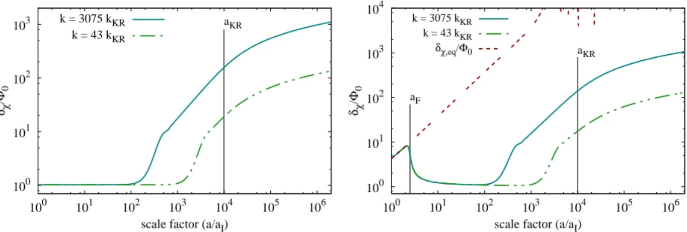
Figure 2.1 shows the evolution of dark matter density perturbations obtained by numerically solving Eq. (2.12) for freeze-in and freeze-out scenarios. The two modes shown in Figure 2.1 both enter the horizon during an era of kination. The two modes have wavenumbers k= 43kKR and
k= 3075kKR, wherekKR≡aKRH(aKR) is the wavenumber of the mode that enters the horizon at
kinaton-radiation equality. The two modes enter the horizon respectively ata= 1300 anda= 150, while kinaton-radiation equality occurs at aKR = 104. In the freeze-in scenarios, the dark matter
density perturbations are initially constant in conformal Newtonian gauge. Since our perturbation evolution starts after pair production has mostly ended, ρχ∝a−3. To ensure that the curvature perturbationζχ= Φ−δχρχ/(aρ0χ) remains constant outside the horizon,δχ must also be constant outside the horizon for freeze-in scenarios. The situation is more complicated for freeze-out scenarios because δχ=δχ,eq until freeze-out, after which δχ decreases toward Φ0 to maintain adiabaticity
before horizon entry.
Once a mode enters the horizon, the dark matter density perturbation experiences a kick from the decaying gravitational potential (see Figure 2.3). After the kick, the dark matter density perturbations grow linearly with the scale factor until kinaton-radiation equality, after which they grow logarithmically. The evolution of dark matter density perturbations is oddly similar during an era of kination and matter domination, in spite of the fact that the pressure of the kinaton forces Φ to evolve very differently during an era of kination. In the following sections, we analytically solve for the evolution of Φ andδχ in order to determine the physical mechanism behind the linear 4