Vol 11, No 3 (2019)

An optimal clustering algorithm-based distance

aware routing protocol for wireless sensor networks

Salim

KHEDIRI

_{, Rehan Ullah Khan}

_{, Waleed Albattah}

1_{Department of Information Technology, College of Computer, Qassim University, Buraidah: 51452, KSA} 2_{Faculty of Science of Gafsa, Department of Computer Science, University of GAFSA, TUNISIA}

Abstract: These Wireless Sensors Networks (WSN) consist of low power devices that are deployed at different geographical isolated areas to monitor physical event. Sensors are arranged in clusters. Each cluster assigns a specific and vital node which is known as a cluster head (CH). Each CH collects the useful information from its sensor member to be transmitted to a sink or Base Station (BS). Sensor have implemented with limited batteries (1.5V) that cannot have replaced. To resolve this issue and improve network stability, the proposed scheme adjust the transmission range between CHs and their members. The proposed approach is evaluated via simulation experiments and compared with some references existing algorithms. Our protocol seemed improved performance in terms of extended lifetime and achieved more than 35% improvements in terms of energy consumption.

Keywords: energy-efficient clustering; Wireless sensor

networks; Improved Artificial bee colony.

1.

Introduction

Wireless Sensors networks is a set of wireless sensor nodes (SNs), self-configured, distributed and autonomous, that detect their physical or surroundings activities like, pressure, temperature or sound in specific area of deployment [1]. A sensor characterized with limited computation capabilities and storage receive the data through analogue to digital converter (ADC). Then, transmit it further for transmission to a central point, known as Base Station (BS) via a wireless connectivity [2], were the data treated for making decision in various applications.

Routing in WSNs is a serious of processes of forwarding information gathered by sensors to the BS. In literature three categories of routing protocols are designed: 1- location-based routing protocols 2- flat routing protocols 3- hierarchical routing protocols [3]. Clustering protocols can perform better than others in term of balancing energy consumption and lifetime prolongation. Generally, with clustering method, the network area is divided into small groups termed as clusters, with a predefined number of leaders known as Cluster Head (CH). All the SNs gathering data and transmit it to their corresponding CH, which finally aggregates it to the BS for additional processing. Clustering has various significant advantages over classical techniques [4]. First, clustering ensure to balance the energy consumption within the network by periodically rotate the role of CH among all nodes. Secondly, data aggregation is applied on data, received from various nodes members within a cluster, to decrease the quantity of data to be transmitted to the BS thus energy requirements decline sharply.

In this paper, we present a new protocol clustering protocol to address the problem of lifetime maximization of WSN. The proposed technique reduces the energy consumption of individual sensor by using the same phenomenon of

propagation is introduced with the advantage of employing fewer control parameters to reduce the unnecessary transmissions and inapt CHs. By prohibiting the unsuitable Chs sensors from participating in the path finding process, unnecessary transmissions are reduced, and network lifetime is maximized. The proposed method demonstrates their proficiency in term of delivery of data packets and network lifetime compared with LEACH, BeeCluster and O-LEACH. The reset of this paper proceeds as follows. Section 2 deals with related work. Section 3 presents the system model. Section 4 deals with the proposed protocol then section 5 presents the simulation results and discussion. Section 6 presents the conclusion.

2.

Energy efficiency protocols: Survey

In the relevant literature, several research works [4] score discuss clustering protocols for fix network, worth mentioning among which one can site: LEACH, BeeCluster, O-LEACH and others.

2.1 Low energy Adaptive clustering Hierarchy (LEACH)

The Low Energy Adaptive Clustering Hierarchy (LEACH) protocol is considered as a guideline of clustering-based routing protocol to extend network lifetime and to achieve scalable solutions [4]. The main idea behind LEACH is to extend lifetime and minimization as possible of global energy usage by the network. The LEACH operation is folded into two principal rounds. Starting with setup phase, the nodes represent the cluster heads have been chosen randomly after distributing all sensor nodes. The elected of Cluster Heads has performed probabilistically at the beginning of each round, defined by a random number chosen between 0 and 1. If this number is less than threshold T(n) (Eq. (1)) that node is selected as a CH for the current round.

𝑇(𝑛) = {

𝑇

1−𝑝(𝑟 𝑚𝑜𝑑 _𝑝1) 𝑖𝑓 𝑛 ∈ 𝐺

0 𝑒𝑙𝑠𝑒

✓ P: is the desired percentage of choosing CHs.

✓ R: is the current round.

✓ G: is the set of sensors nodes that have not been cluster heads in last 1/p rounds.

Secondly the steady phase, responsible for data transfers to the sink node. Each sensor member transmits data during its own time-slot and reduces energy consumption by entering sleep mode during the remaining time-slots. Each cluster head has its own time to aggregates data in the designated slot and sends them to the sink.

✓ Setup phase ✓ Steady-state phase 2.2 I-LEACH

Recently, a new clustering algorithm called I-LEACH (Improvement of LEACH) it has proposed by Kumar and Kaur [5], was designed to prolong lifetime of the network with two changes. The CH selection criterion involves the nodes based on its energy reserve secondly uses coordinates for cluster formation to guarantee that at least.

2.3 DWEHC

DWEHC [6] (Distributed Weight-Based Energy-Efficient Hierarchical Clustering) is also a good example of effective clustering algorithms. The reporting phase of the different CH's is similar to that of HEED. In fact, the choice of CHs is made according to the energy reserve and the degree. Intra-cluster communication is performed in k-jumps and is limited by a well-defined range. Each member node then looks for the least expensive path to its CH. This procedure and the limitation of the number of intra-cluster jumps have minimized the energy consumption of this algorithm by comparing it to that of HEED.

2.4 EELBC

EELBC [7] is a centralized algorithm where the BS handles the clustering procedure. The first step is to arrange the gateways according to the number of nodes restricted (nodes that communicate with a single gateway). Then, each node is connected to the nearest gateway. EELBC has shown its effectiveness by comparing with LBC in terms of energy consumed and number of dead nodes.

2.5 TL-LEACH

In Loscri et al, have proposed Two Level Hierarchy LEACH (TL-LEACH) [8], which presents an extension of the LEACH algorithm. TL-LEACH Uses the following techniques to achieve energy efficiency: random, adaptive and auto-configuration for clustering location control is also proposed for data transfers. In TL-Leach, a cluster-head receives data from its members like LEACH, but instead of transmitting data to the base station directly, it uses some of the clusters-heads that lies between the cluster-head and the base station as relay points. TL-LEACH presented a two-level hierarchy: top clusters-heads called (CHi) primary, and a second level called secondary cluster-heads (CHij). The algorithm consists of four main phases: advertisement phase, cluster setup phase, schedule creation and phase data transmission.

2.6 BeeCluster

The BeeCluster [1], based on an iABC meta-heuristic which uses first of its kind Student's-t cPDF and DE inspired improved solution search equation ABC/rand- to-opt/1 to improve exploitation capabilities as well as convergence rate of existing ABC meta-heuristic. BeeCluster uses an energy-efficient approach, which selects optimal CH's based on an improved search equation and an efficient fitness function. 2.7 O-LEACH

In [13], the authors proposed O-LEACH algorithm, cross-layer optimization problem based on LEACH protocol. O-LEACH uses same practice of O-LEACH to select the cluster-heads and cluster formation. But, O-LEACH process more life span of nodes. This is because, during the cluster-heads selections uses residual energy with a defined threshold

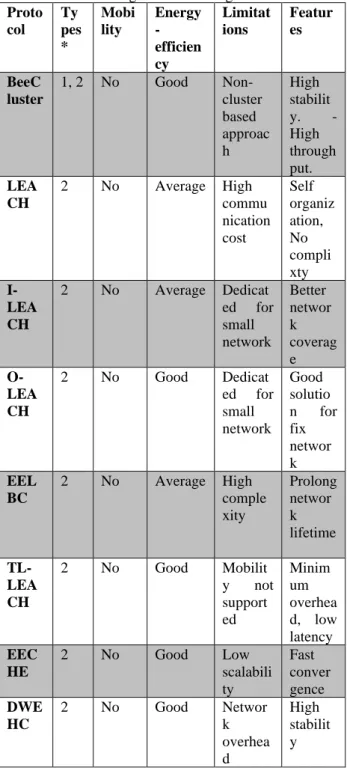
value. Below in table I, we introduce a relative comparison of these protocols, highlighting their features and limitations for a better insight.

2.8 EECHE

Kumar et al, have proposed the EECHE protocol, Energy Efficient Cluster Head Election Protocol [9], used for heterogeneous sensor networks. The authors assumed that all nodes are uniformly distributed and some nodes have additional energy. Kumar et al used three types of nodes. Type 2 nodes are nodes that have more energy than $type-1$ $(in quantity of α times) and type 3 nodes that have more energy than type-1 $nodes (in quantity of  time ). E0 is the initial energy of the type 1 nodes, while the energy of the type 3 and type 2 nodes are respectively:E0 = (1 + ) et E0 = (1 + ).

Table 1. comparison of various clustering approaches * : 1-Heterogenous/2-Homogenous. **. Proto

col Ty pes *

Mobi lity

Energy -efficien cy

Limitat ions

Featur es

BeeC luster

1, 2 No Good

Non-cluster based approac h

High stabilit

y.

-High through put. LEA

CH

2 No Average High commu nication cost

Self organiz ation, No compli xty

I-LEA CH

2 No Average Dedicat ed for small network

Better networ k coverag e

O-LEA CH

2 No Good Dedicat

ed for small network

Good solutio n for fix networ k EEL

BC

2 No Average High comple xity

Prolong networ k lifetime

TL-LEA CH

2 No Good Mobilit

y not support ed

Minim um overhea d, low latency EEC

HE

2 No Good Low

scalabili ty

Fast conver gence DWE

HC

2 No Good Networ

k overhea d

The following table (table 1) depicts a comparison of all the protocols presented above according to several criteria (data transmission, type of networks, energy efficiency, mobility, etc.). As sensor networks are applied in various fields, we have selected different parameters depending on the applications where they can be applied. Detailed analysis of all LEACH-based routing and clustering protocol variants against various parameters are given below in Table 1. The different parameters selected for the next discussion are data transmission, network type, routing type, deployment strategy, energy efficiency, scalability, scalability, mobility, reliability and communication. Regarding data transmission, either single-hop or multi-hop communication between nodes in sensor networks were considered. Most existing protocols use multi-hop communication between nodes, TL-Leach uses two-hop communication. The sensor nodes in most protocols are classified as either homogeneous or heterogeneous depending on the different energy levels of nodes. I-LEACH, EECHE, used heterogeneous nodes while the rest of the protocols took homogeneous nodes. Nodes that are heterogeneous in nature adjust to different levels for data transmission and performing various other operations to save energy. To reduce the amount of energy of the sensor nodes, the majority of the protocols used the clustering method from which the simple nodes communicate with a CH's node and then it is last transferred these data to the Base Station (BS). One of the nodes can be elected as CH according to various parameters in order to save the energy of the nodes. Most protocols used the random deployment of nodes except W-Leach in which it uses both the uniform and non-uniform node deployment was considered. The deployment of sensor nodes is used to estimate the coverage and connectivity of nodes which is an important factor to study. This is because some of the nodes may be located in the corners of the deployment area and have poor connectivity with the CH's if these nodes may not be able to transmit the data collected to the respective CH's and base station.

Generally, the BS in the sensor networks is considered static. But the BS can also be considered mobile in this case, maintaining the mobile SB creates an additional load in the network that results in more power consumption in the network. Keeping in view of the above, only a few proposals have examined the mobility of SB. When performing any operation, sensor nodes use radio links to transfer data from CH to SB, so that some communication costs also occur during this process. For scalability this factor is essential because the number of nodes changes frequently, it can go from a hundred to thousands. The routing protocols must therefore be very scalable. In other words, routing protocols should be efficient regardless of the number of nodes. It must adapt to the change in density of the network. Depending on the data size and available bandwidth, the cost of communication may vary from very low, low, medium, and high.

3.

Model and Assumption

In this section, the network model, energy usage model and other assumption are considered. We have tried to develop our clustering model on a realistic scenario [13], [14].

3.1 Network model

We modeled the proposition scheme by a Euclidean graph G=(V, E), where V is the set of sensors and E={(u,v)  V/D(u,v)<=R} represents the wireless connections between nodes. R is the transmission range and D(u,v) denotes the Euclidian distance between the node u and the node v. 3.2 Energy model

To ensure the comparison with previous works [10,11,12] the authors have used the simple model for the radio energy dissipation model where the transmitter dissipates energy

ETX(k,d) to run the radio electronics and the power amplifier.

The receiver dissipates energy ERX(k) when managing the

radio electronics, as shown in fig.1.

Figure 1. Radio energy dissipation model [13]

the necessary energy consumption for transmission of l bits is composed of three parts : the energy consumed by the transmitter Etrans, by the receiver Erec and by the ACK packet exchange Eack :

)

2

(

)

,

(

)

,

(

)

,

(

total

l

d

E

l

d

E

l

d

E

E

=

+

+

The energy consumed for transmitting l bits of data is given by :

)

3

(

)

,

(

.

)

,

(

l

d

l

E

E

l

d

E

=

+

further, if the distance between transmitter, and receiver is d, then :

)

4

(

where the equation signifies the threshold distance and the energy electronics. To receive l bit message, the radio spends Erec(l,d) as follows :

Erec(l,d)= l*Eelec

(5)

Energy consumed for ACK packet exchange is calculated according to eq (6).

)

6

(

)

(

ack

ack

E

E

E

=



+

where is the ratio between length of acknowledgement packet to data packet.

We begin by briefly discussing some key concepts and notation relevant to the models presented in this paper 3 S is the set of sensor nodes S = { s1, s2, ...sn}, which are

randomly distributed over a geographical area of defined dimensions m × m, whereas sn+1 denotes the

BS. Each sensor node has a communication radius r. 4 L is the set of bidirectional wireless links between two

sensor nodes, where li,j ∈ L represents wireless link between node si and sj.

Etrans(l,d)=

lEelec+lefsd2 if d<d0

lE_elec+lempd4 _{if d³d}

0 (4)

ì

í ïï

î ï ï

d

=

e

e

t

=

l

5 Set of Cluster Heads (CH's) are denoted by Sch = { ch1,

ch2, ...chk} where Sch ∈ S.

6 Dsisj(max) represents the maximum distance between a

senor node si 
and sj which is calculated by squared

Euclidean distance between them as 
Dsj_{(max)=Max{dis(s,s)} | ∀ s}

i, 

sj ∈ S=∥si

−sj ∥2 _{= ∑(si −sj)}2 _{|∀si,sj ∈S}

₍₇₎

7 Dsn+1_{(max) specifie the maximum distance between a}

senor node si i 
and BS which is calculated by squared

Euclidean distance between them as 
 Dsn+1_{(max) = Max{ dis(s}

i, 
sn+1)} |∀si

∈S=∥si−sn+1∥2_{=∑(si−sn+1)}2 _|∀s

i∈S

(8)

8 Dchj_{(max) presente the maximum distance between a}

senor node si 
and cluster head chj which is calculated

by squared Euclidean distance between them as Dchj_{(max)=Max{dis(s}

i,chj)} | ∀ s, chj ∈S=∥si −chj ∥2 = ∑(si

−chj)2 _{| ∀ s}

i, chj ∈S

(9)

9 represents the maximum distance

between a cluster-head chj and BS, is calculated by

squared Euclidean distance between them as 10



=

− =  

+

+ +

+

ch n

j

n j ch n

j S

ch

S j s

ch

s ch S S

ch dis D n

j

| ) (

| )} , ( (max){

2 1

2 1 1

1

(10)

If there will be n nodes uniformly distributed in an m*m field with k clusters, then there will be n nodes per cluster. Out of these, there will be one CH node and remaining non-CH nodes. Now energy consumed by a non-non-CH node is given by:

)

11

(

)

,

(

)

,

(

l

d

E

l

d

E

=

)

12

(

)

,

(

*

)

,

(

l

d

l

E

E

l

d

E

=

+

and energy consumed by a CH node is given by: ) ) 1 ( * *

* ) 1 ( ) , ( ) ,

( trans elec da ack

ch E

k n E l k n E l k n d l E d l

E = + − + + −

)

13

(

where Eda is the energy consumed by CH for data

aggregation at its end.

Now, the total energy consumed in a cluster is given by:

ch non ch

cluster

E

k

n

d

l

E

E

=

(

,

)

+

(

−

1

)

(

14

)

Therefore, energy consumed in whole network per round is given as:



=

j

cluster

round

E

j

E

1

)

(

(

15

)

4.

Proposed PC-LEACH

As can be seen in fig.2, in our cluster formation phase, we used the principle of wave propagation, where the propagation starts from the center until the limit of surface. First, we assumed that N nodes are deployed uniformly in the square zone of 100m*100m and the base station coordinates are (50, 50) as shown in fig 5 below.

Figure 2. one round of the clustering process

4.1 Cluster head selection phase

The proposed protocol is described in figure (3). The clustering is break into stages: The first CH selection cluster formation, data aggregation and data communication. As illustrated in fig 5. The setup state clenched by CH selection and proceeds by cluster formation. The later state is followed by the data transmission state which is divides into data aggregation and data communication. Therefore, the first step is the election of cluster head with the closest nodes to the BS. In the second step, the election of CH is made by the first elected CH, after recursively repeating this phenomenon. The node immediately transmits its CH status its neighbor nodes by broadcasting a cluster head advertisement message. After the selection of cluster head, we must wait the belonging of the member nodes into the cluster. Behind clusters organization, each cluster head creates its TDMA table and transmit it to different nodes, then uses the CDMA technique to transmit data captured to the BS.

Figure 3. Flowchart for operation of PC-LEACH ▪ BS Initiation of the routing process by the BS

▪ Election of CH in the first rounf with mean distance with the BS. Election of a CH in the second round with mean distance from the first elected CH and generation of their members.

▪ This process with iterative procedure until reaching the final CH (fig.4).

D

sn+1

▪ Repetition of the iterative process until draining energy of all sensors.

▪ After selection of the head, wait for member’s nodes. ▪ Creation of the table TDMA and send it to the

members.

▪ Launching of the transmission phase.

Figure 4. The process of the elected CH of PC-LEAC

5.

Simulation Results and discussion

In this section, the performance of proposed protocol is evaluated and compared with the conventional clustering protocols of BeeCluster, O-LEACH and LEACH. The simulation was performed using Matlab 2014 a tool under a range of conditions.

5.1Simulation Environment

In order to validate the analytic model described in the previous sections a simulation scenario is provided here. All simulation was performed using Matlab software. We consider N nodes number varies between 50 and 100 nodes randomly deployed in a topological area of dimension 100 x 100 m2. We assume that the base station is located at the center of the sensing region.

In this scenario, to compare the performance of Optimum-LEACH with those of the Optimum-LEACH protocol, we performed the simulations in execution contexts different. Thus, in order to analyze the robustness of our approach in relation to the number of nodes, we have chosen to evaluate the following metrics and compare them with those from LEACH.

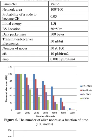
The average lifetime of the network (with 100 nodes), The results obtained for these metrics are presented in Figures 4, 5 and 6 (with 5\% of the nodes as CHs).

The network is organized into a clustering hierarchy, and the cluster-heads execute fusion function to reduce correlated data produced by the sensor node within the clusters. Parameters settings for Optimum LEACH can be summarized in Table II. To avoid the frequent change of topology, we assume that the nodes are in static mode; the protocol compared with Multihop-LEACH , O-LEACH and LEACH.

The two graphs Fig.4 and fig.5 , it can be noted that the performance of PC-LEACH maintains the network operational lifetime of more than 5000, 4000, 4200, 4600 more than LEACH, O-LEACH and Beecluster respectively for 100 nodes, the fascinating results is that under the most dense network that containing 300 sensors, our PC-LEACH gives extremely high value of 4600 rounds compared with

3200, 4100, 4250 round of LEACH, O-LEACH and BeeCluster respectively. This indicate that as the network size increase the performance of PC-LEACH continues to improve.

Table 2. Simulation Parameters

Parameter Value

Network area 100*100

Probability of a node to

become CH 0.05

Initial energy 1.5j

BS Location 50*50m

Data packet size 500 bytes Transmitter/Receiver

Electronics 50 nJ/bit

Number of nodes 50 & 100

εfs 10 pJ/bit/m2

εmp 0.0013 pJ/bit/m4

Figure 5. The number of alive nodes as a function of time (100 nodes)

Figure 6. The number of alive nodes as a function of time (300 nodes)

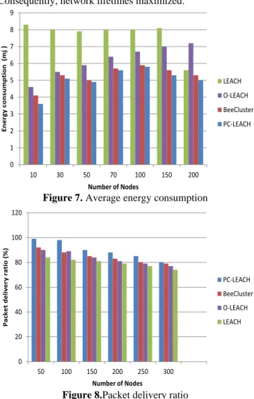
Figure 6 represents the energy consumption and depicts that PC-LEACH reduced energy consumption for each case and always yielded lower values than others and is more effective in saving energy than BeeCluster, O-LEACH and LEACH reduce between 0% and 35% of energy consumption.

We are also interested in the impact of the number of packet delivery. Fig. 7 shows that PC-LEACH delivers highest number of packet among its all peers, even at highest density of nodes. This is due that, each time a packet is sent, LEACH, BeeCluster, and O-LEACH always select node with less energy for each packet transmission that results in

0 20 40 60 80 100 120

500 2000 2500 3500 4000 4500 5000

N

u

m

b

er

o

f

al

iv

e

n

o

d

es

(

10

0)

Number of Rounds

PC-LEACH BeeCluster O-LEACH LEACH

0 50 100 150 200 250 300 350

500 2000 2500 3500 4000 4500 5000

N

u

m

b

e

r

o

f

al

iv

e

n

o

d

e

s

(

3

0

0

)

Number of Rounds

an early dead situation of the nodes. But in our case, proposed algorithm selects a strong node in term of energy to transmit the packets. Thus, the load is distributed among the maximum number of sensor nodes in the network. Consequently, network lifetimes maximized.

Figure 7. Average energy consumption

Figure 8.Packet delivery ratio

6.

Conclusion

The routing mechanisms is a phenomenon subject to many constraints which must meet several requirements. These constraints sometimes can be contradictory such as maximizing the number of sent information and the quality and accuracy of service provided and minimizing energy consumption.

In this paper, we proposed a new static clustering algorithm extended LEACH algorithm, to enhance WSN performance in terms of energy consumption, Packets delivery and lifetime. Thereafter, we compared our proposed algorithm with most known clustering algorithm like BeeCluster, PEGASIS and LEACH.

Nevertheless, the remains a great need for further research related to the impact of deployment of heterogeneous nodes having high energy capacity and others factors to select CHs.

References

[1] P. S. Mann, & S. Singh, “Improved metaheuristic based energy-efficient clustering protocol for wireless sensor networks”. Engineering Applications of Artificial Intelligence, 57, 142-152, 2017.

[2] MA. rghavani, M.Esmaeili, F.Mohseni, & A. Arghavani, “Optimal energy aware clustering in circular

wireless sensor networks”. Ad Hoc Networks, 65, 91-98, 2017.

[3] K..Akkaya & M. A.Younis, “survey on routing protocols for wireless sensor networks”. Ad hoc networks, 3(3), 325-349, 2005.

[4] H.Shin, S. Moh, I.Chung & M.Kang, “Equal-size clustering for irregularly deployed wireless sensor networks”. Wireless Personal Communications, 82(2), 995-1012, 2015.

[5] N.KUMAR et J. KAUR, “Improved leach protocol for wireless sensor networks”. In : Wireless Communications, Networking and Mobile Computing (WiCOM) 7th International Conference on. IEEE, 2011. p. 1-5, 2011.

[6] P.DING, J. HOLLIDAY, et A. CELIK,. “Distributed energy-efficient hierarchical clustering for wireless sensor networks”. In : International conference on distributed computing in sensor systems. Springer, Berlin, Heidelberg, p. 322-339, 2005.

[7] P. KUILA et K. JANA, “Energy efficient load-balanced clustering algorithm for wireless sensor networks. Procedia Technology”, vol. 6, p. 771-777, 2012.

[8] V.Loscri, G. Morabito, & S.Marano, “A two-levels hierarchy for low-energy adaptive clustering hierarchy (TL-LEACH)”. In Vehicular Technology Conference. VTC-2005-Fall. 2005 IEEE 62nd (Vol. 3, pp. 1809-1813). IEEE, 2005.

[9] K. Abido, Dilip, T. C.ASERI, et R. PATEL, B. EECHE: “energy-efficient cluster head election protocol for heterogeneous wireless sensor networks”. In : Proceedings of the international conference on advances in computing, communication and control. ACM, p. 75-80, 2009.

[10] Z.Yong, & Q.Pei, “A energy-efficient clustering routing algorithm based on distance and residual energy for wireless sensor networks”. Procedia Engineering, 29, 1882-1888, 2012.

[11] M. Aissa, A. Belghith & K. Drira.”New strategies and extensions in weighted clustering algorithms for mobile ad hoc networks”. Procedia Computer Science, 19, 297-304, 2013.

[12] N. Nasri, A. Ben Fradj, & A. Kachouri, “Optimised cross-layer synchronisation schemes for wireless sensor networks”. International Journal of Electronics, 104(7), 1178-1189, 2017.

[13] S. El Khediri,N. Nasri, A. Wei, & A. Kachouri, “Probabilistic Energy Value for Clustering in Wireless Sensors Networks”. Wireless Sensor Network, 5(2), 26, 2013.

[14] O. Dina, & M. Ahmed kheder, “SEPCS: Prolonging Stability Period of Wireless Sensor Networks using Compressive Sensing”. International Journal of Communication Networks and Information Security (IJCNIS),2019.

0 1 2 3 4 5 6 7 8 9

10 30 50 70 100 150 200

E

n

e

rg

y

c

o

n

su

m

p

ti

o

n

(

m

j

)

Number of Nodes

LEACH

O-LEACH

BeeCluster

PC-LEACH

0 20 40 60 80 100 120

50 100 150 200 250 300

P

a

ck

e

t

d

e

li

v

e

ry

r

a

ti

o

(

%

)

Number of Nodes

PC-LEACH

BeeCluster

O-LEACH