Fuzzy multi-objective optimization of linear functions subject to max-arithmetic mean relational inequality constraints

Sharif University of Technology

Transactions E: Industrial Engineering www.scientiairanica.com

Fuzzy multi-objective optimization of linear functions

subject to max-arithmetic mean relational inequality

constraints

F. Kouchakinejad

_{, M. Mashinchi}

_{and E. Khorram}

a. Department of Mathematics, Graduate University of Advanced Technology, End of Haft Bagh-e-Alavi Highway, Kerman, Iran. b. Department of Statistics, Faculty of Mathematics and Computer Science, Shahid Bahonar University of Kerman, Pajohesh

Square, 22nd Bahman Blvd, Kerman, Iran.

c. Faculty of Mathematics and Computer Sciences, Amirkabir University of Technology, 424 Hafez Ave, Tehran, Iran. Received 27 June 2015; received in revised form 2 March 2016; accepted 26 April 2016

KEYWORDS Fuzzy inequality; Fuzzy relational inequalities; Fuzzy solution; Linear objective function;

Max-arithmetic mean composition;

Multi-objective optimization.

Abstract. The main goal of this work is to nd a better solution to a kind of multi-objective optimization problem subject to a system of fuzzy relational inequalities with max-arithmetic mean composition. First, this problem is solved and, then, in the case that the decision maker is not satised with any of the solutions, by assigning linear membership functions to the inequalities in the constraints and objective functions and using Bellman-Zadeh decision, a new solution is found. This new solution does not belong to the feasible domain but is considered acceptable based on the decision maker's view. In order to nd this solution easier, some simplication processes are given. Afterwards, an algorithm is presented to generate the new solution. Finally, an example is given to illustrate the steps of the algorithm.

© 2017 Sharif University of Technology. All rights reserved.

1. Introduction

Since the time the notion of Fuzzy Relational Equation (FRE) was introduced by Sanchez, many works have been done in the domain of FREs, Fuzzy Relational Inequalities (FRIs), and the problems relevant to them; for instance, see Khorram and Zarei [1], Yang [2], and Zhou et al. [3]. The usage of FREs and FRIs can be observed in many elds such as fuzzy control, fuzzy decision making, knowledge engineering, image processing, image and video compression and decom-pression, image reconstruction, fuzzy modeling, fuzzy diagnosis, and especially fuzzy medical diagnosis [4].

*. Corresponding author. Tel./Fax: +98 34 33357280 E-mail addresses: [email protected] (F. Kouchakinejad); [email protected] (M. Mashinchi); [email protected] (E. Khorram)

Max-min composition is the most frequently used composition in FREs and FRIs. Nevertheless, it is shown that the min operator is not always the best selection for the intersection operation [5]. Thus, some researchers have studied FREs and FREIs in the presence of other compositions. For example, Molai [6] and Hassanzadeh et al. [7] considered max-product composition, whereas Khorram et al. [8] and Guu et al. [9] employed max-t-norm composition in their problems. For the rst time, Zimmermann used the arithmetic mean operator, which was not a t-norms as an \and" operator. Following Zimmermann's idea [10], Khorram et al. [1,5] and Wu [10] considered FREs and FRIs under max-arithmetic mean composition. In [4], it was shown that with regards to sensitivity, the arithmetic mean was one of the best aggregation operators. Thereafter, a fuzzy optimization problem

subject to a system of max-arithmetic mean relational inequality was studied.

In addition to problems in which an objective function is optimized over a system of FREs or FRIs, multi- objective optimization problems have been con-sidered by some researchers [8,9]. In [1], a multi-objective optimization problem in the presence of a system of FREs with max-arithmetic mean composi-tion has been considered. In [11], the authors have studied the same problem with FRIs.

As it is mentioned in [12], when the Decision Maker (DM) is not satised with the solution of an optimization problem, it is possible to soften the rigid requirements of the DM in order to consider the im-precision of his/her judgment so that a better solution can be obtained. To pursue this idea, in [13], the authors have considered the fuzzy linear optimization problem in the presence of fuzzy relational inequality constraints with max-min composition. Also, in [4], this problem has been studied with max-arithmetic mean composition. To the authors' best knowledge, no work has been done to investigate the multi-objective model of the problem which has been studied in [4]. Here, we study this kind of problems.

As an application of this model, we can consider the given example in [13]. Consider a schoolmas-ter who decides to cover three educational zones by enhancing the educational quality of his school (A). He considers some criteria to convince the parents to select school A. Also, he has some plans for each potentially poor criterion. Thus, he wants to resolve the problem of parents as desirably as possible in three zones by enhancing the quality such that they prefer to select school A while the cost expended for this purpose becomes less than or equal to the budget. In the case that the schoolmaster has more aims such as maximizing the spent budget for one of the criteria (consider athletic-recreational facilities that can be considered as a potential investment for the school) in comparison to other expenses, we have a multi-objective problem subject to a system of fuzzy relational inequalities. This problem can be considered with any max-aggregation function composition. As we have shown in [4], one of the best choices for an aggregation function to use in FRIs is arithmetic mean, which is the chosen aggregation function of this paper. The rest of the paper is outlined in the following. In Section 2, a multi-objective optimization of linear functions with ordinary inequalities in the presence of a max-arithmetic mean composition problem is studied [11]. Then, using a selected solution and linear membership functions, the multi-objective optimiza-tion problem in the presence of the fuzzy inequalities is converted into another problem with one objective function. In Section 3, the main goal is to reduce the dimension of the feasible domain as much as

possible. Section 4 introduces an algorithm to give the solution using the steps of Section 3 and provides one numerical example to illustrate the algorithm. Concluding remarks are given in Section 5.

2. Problem formulation

Consider the following linear multi-objective optimiza-tion problem:

min fZ1(x); ; Zp(x)g;

s.t. A x b;

x 2 [0; 1]n_{: (1)}

where, \" stands for the max-arithmetic mean com-position. Assume that DM is not satised with (any of) the solution(s) of Relation (1). In this case, we try to nd a better solution, which is called fuzzy solution here. Fuzzy solution, which violates at least one constraint and is still acceptable to be a solution based on the DM's view, is achieved by softening the constraints of Relation (1) [13]. The amount of perturbations imposed on the constraints is determined by having interaction with the DM. To this end, the focus is on solving the following problem:

g

min fZ1(x); ; Zp(x)g;

s.t. A x 4 b;

x 2 [0; 1]n_{; (2)}

where, A = (aij)mn is a matrix, and b = (bi)m1

and x = (xj)n1are the right-hand-side and unknown

vectors, respectively, such that aij, bi 2 [0; 1]; i 2

I = f1; 2; ; mg and j 2 J = f1; 2; : : : ; ng. Also, for all l 2 L = f1; 2; ; pg, Zl(x) = ctlx are linear

objective functions where, cl = (clj)n1, clj 2 R and

R is the set of real numbers. Here, \gmin" and \4" represent moderate or fuzzy types of \min" and \6" meaning that \objective functions should be minimized as much as possible" and \the constraints should be well satised", respectively [12].

Let ai denote the ith row of matrix A; then,

Relation (2) can be demonstrated as follows: g

min fZ1(x); ; Zp(x)g;

s.t. ai x 4 bi; i 2 I;

x 2 [0; 1]n_;

where, ai x 4 bi means maxj2J(aij₂+xj) 4 bi for all

i 2 I.

In order to solve Relation (2), it is necessary to nd solutions of Relation (1); then, dene member-ship functions for 4 and objective functions; and use

Bellman-Zadeh decision [14]. Accordingly, Relation (1) and its solutions have a signicant role in solving Relation (2). Correspondingly, in the following, some previously obtained results are stated [4,5,11,12] that are in the direction of solving Relation (1).

Notation 1 [4]. Set: Si_{(A; b) = fx 2 [0; 1]}n_{: a}

i x big for all i 2 I;

S(A; b) =\

i2I

Si_{(A; b) = fx 2 [0; 1]}n_{: A x bg:}

Denition 1 [12]. bx 2 S(A; b) is a complete optimal solution to Relation (1) if and only if Zl(bx) Zl(x),

for all l 2 L and all x 2 S(A; b).

Nevertheless, generally, when the objective func-tions conict with each other, such a complete optimal solution which concurrently minimizes all of the objec-tive functions does not always exist. Therefore, Pareto optimal solution is used as a substitute [12].

Denition 2 [12]. x0 _{2 S(A; b) is said to be a Pareto}

optimal solution to Relation (1) if and only if there does not exist another x 2 S(A; b) such that Zl(x) Zl(x0)

for all l 2 L and Zl(x) 6= Zl(x0) for at least one l.

Throughout this work, any kind of (com-plete/Pareto) solution is called an \optimal solution". However, it is clear that a complete (Pareto) optimal solution yields a fuzzy complete (Pareto) optimal solu-tion.

The following theorems state some properties of S(A; b). For more details and proof of theorems see [4,5].

Theorem 1 [4].

a) S(A; b) 6= ;, if and only if for all i 2 I and all j 2 J, 2bi aij > 0;

b) If S(A; b) 6= ;, then 0 = [0; 0; ; 0]t

1n is the

unique minimal element of S(A; b).

Theorem 2 [4]. If S(A; b) 6= ;, then x = (xj)n1

is the unique maximal element of S(A; b) where, xj =

minf1; mini2If2bi aijgg.

Here, the feasible domain of Relation (1) can be given.

Corollary 1. If S(A; b) 6= ;, then S(A; b) = [0; x]. Now, one simplied form of Relation (1) can be presented.

Theorem 3. Relation (1) is equivalent to the fol-lowing problem:

min fZ1(x); ; Zp(x)g;

s.t. x 20; x: (3) Proof. Due to Corollary 1, the proof follows immediately.

Notation 2. Set: J0_{= fj 2 Jjc}

lj< 0 for all l 2 Lg;

J00_{= fj 2 Jjc}

lj > 0 for all l 2 Lg;

J = J n (J0_{[ J}00_{) and}

J_{= J n J}00_:

Theorem 4. If xos is an optimal solution to

Rela-tion (3), then (xos)j = xj and j 2 J0 and (xos)j = 0

for all j 2 J00_.

Proof. Let x 2 S(A; b) be an optimal solution where, for some j0 _{2 J}0_{, x}

j0 6= x_j0. Set x0_j = x_j for all j 2

J n fj0_{g and x}0

j0 = x_j0. Thus, Z_l(x0) < Z_l(x) for all

l 2 L, which is a contradiction. Similarly, the other part could be proven.

According to Theorem 4, it is enough to compute (xos)jfor all j 2 J. Thus, in order to solve Relation (3)

and, as a result of Theorem 3 to solve Relation (1), we just consider the following problem:

min X

j2J

cljxj+

X

j2J0

cljxj for all l 2 L;

s.t. xj 2 [0; xj] for all j 2 J: (4)

Since the feasible domain of Relation (4) is no longer a system of FRIs, it can be solved by any existing method for these kinds of problems that are explained in [12]. Also, it can be solved by heuristic methods such as the Genetic algorithm [15]. If the problem has several solutions and the DM is satised with none of them, then the DM shall choose one of these solutions based on his/her point of view in order to obtain one fuzzy solution [11].

Now, using the selected solution of Relation (1), we try to solve Relation (2). In fact, we are going to investigate if it is possible to minimize all objective functions considering aspiration levels zlof the DM by

imposing certain exibility on the constraints. That means we consider the following problem:

ct

lx 4 zl; for all l 2 L;

A x 4 b;

x > 0: (5)

acceptable exibility on the constraints are specied having interaction with the DM. Then, the following linear membership functions for fuzzy inequalities in Relation (5) can be employed as in [4,13]:

i(ai x) =

8 > < > :

1 ai x 6 bi

1 aix bi

di bi6 ai x 6 bi+ di

0 ai x > bi+ di;

(6)

l(ctlx) =

8 > < > :

1 ct lx 6 zl

1 ctlx zl

dl

0 zl6 c

t

lx 6 zl+ dl0

0 ct

lx > zl+ dl0:

(7)

where, zl = Zl(xos) vdl0 for some xed v 2 (0; 1).

Each di and dl0 is a chosen constant expressing the

limit of the permissible violation of the ith inequality for all i 2 I and all l 2 L. Further, l(zl) = 1,

l(Zl(xos)) = 1 v, and l(Zl(xos) + (1 v)dl0) = 0

for all l 2 L. The parameters v, dl

0, and di for all

i 2 I and l 2 L can usually be found based on the empirical-technical views of the DM. Note that Eqs. (6) and (7) allocate a higher degree to those points that are closer to the feasible solution set. Assignment of these membership functions is crucial to nd the best fuzzy solution as near as possible to the feasible solution set. On the occasion that the exibility of the constraints is not sucient, the optimal solution will not change and, afterwards, more exibility is enforced on the constraints to nd a better fuzzy solution [13]. Remark 1 [12]. Some other membership functions can be used, such as piecewise, exponential, hyperbolic, or hyperbolic inverse ones, besides the linear member-ship function.

Notation 3 [13]. Set S = fx 2 [0; 1]n : x =2

S(A; b)g.

In fact, only the vectors of x 2 [0; 1]n _{can be}

better solutions than xosfor Relation (5) that violate at

least one inequality ai x 6 bi. That is, x is an

infeasi-ble solution or, by Notation 3, x 2 Sequivalently [13].

The next theorem represents the most important problem of Section 2.

Theorem 5. Relation (5) is equivalent to the fol-lowing problem:

max ;

s.t. Di

max

j2J(aij+ xj)

+ Bi; i 2 I;

Dl

0(ctlx) + Bl0; l 2 L

x 2 [0; 1]n_{: (8)}

Proof. Similar to [4,12,13], following the decision of Bellman and Zadeh, Relation (5) has the following form:

= max

x2[0;1]n

min

l2L

l(ctlx); min_i2I i(ai x)

: (9)

Considering Eqs. (6) and (7) and substituting Di =2d1i

and Bi = 1+b_di_i for all i 2 I, Dl0=d1l 0 and B

l

0= 1+dzll 0,

Eq. (9) is rewritten as:

= max

x2[0;1]n

( min

l2L

( Bl

0 D0l(ctlx);

min

i2I

Bi Di

max

j2J(aij+ xj)

))

: (10)

Now, by introducing as the auxiliary variable:

=min

l2L

Bl

0 D0l(ctlx); min_i2I

Bi Di

max

j2J(aij+xj)

;

we have: Bi Di

max

j2J(aij+ xj)

; (11)

for all i 2 I and Bl

0 Dl0(ctlx); (12)

for all l 2 L. Using Relations (11) and (12), Problem (8) is equivalent to the following problem:

max ;

s.t. Bi Di

max

j2J(aij+ xj)

; i 2 I

Bl

0 Dl0(ctlx); l 2 L

x 2 [0; 1]n_{: (13)}

Now, from Problem (13), Problem (8) is derived immediately.

Therefore, according to Theorem 5, in order to nd the fuzzy solution to Relation (2), it is adequate to consider Relation (8). In the next section, the dimension of Relation (8) is reduced as much as possible.

3. Simplication process

In this section, some theorems are given in order to convert Relation (8) into the equivalent problems that are more simplied and more easily solvable as well. Similar to [4], we use the following notations:

Notation 4. Set l

0(x) = B0l D0l(ctlx) for all l 2 L;

i(x) = Bi Di

max

j2J(aij+ xj)

for all i 2 I;

ij(xj) = Bi Di(aij+ xj) for all

i 2 I and j 2 J and

(x) = min

min

i2Ifi(x)g; minl2Lf l 0(x)g

:

Theorem 6. The functions i for all i 2 I and ij

for all i 2 I and j 2 J are non-increasing continuous functions. Especially, ijdecreases for each component

xj2 [0; 1]. Also, l0 for all l 2 L decreases with respect

to component xj if cj> 0, and increases if cj< 0.

Proof. Straightforward.

The next theorem provides a simplication pro-cess to solve Problem (8) by nding some components of its solution.

Theorem 7. If x _{is the optimal solution of}

Prob-lem (8), then x

j = 0 for all j 2 J00.

Proof. The proof is similar to that of Theorem 2 in [13].

Remark 2. According to Theorem 7, in the solving procedure of Problem (8), some columns of matrix A can be removed. Thus, to solve Problem (8), it is adequate to consider only the columns of matrix A that belong to J_.

By Remark 2, Problem (8) is converted into the following simplied form:

max ;

s.t. Di

max

j2J(aij+ xj)

+ Bi; i 2 I

Dl 0

0 @X

j2J

cljxj

1

A + Bl

0; l 2 L

x 2 [0; 1]jJ_j

; (14)

where jJ_{j is cardinality of J.}

Theorem 8 [4]. For all i 2 I and j 2 J_,

a) If 2bi aij > 1 then, ij(xj) > 1 for all xj2 [0; 1];

b) If 2bi aij < 1 then, ij(xj) > 1 for all xj 2

[0; 2bi aij].

Proof. See the proof of Theorem 7 in [4]. Theorem 8 has two interesting conclusions. Corollary 2 [4]. Let i 2 I and j 2 J_{. Then,}

ij(xj) > 1 for all xj 2 [0; 1] if and only if xj does

not violate the inequality aij x 6 bi.

Proof. See the proof of Corollary 3 in [4].

Corollary 3 [4]. Under the simplication burdened by Remark 2, x 2 S if and only if there exist i 2 I

such that i(x) < 1.

Proof. See the proof of Corollary 4 in [4].

The next theorem introduces another simplica-tion to convert Relasimplica-tion (14) to the more simplied form.

Theorem 9 [4]. Suppose that the simplication by Remark 2 is done and i 2 I. Then, i(x) =

minj2J

ifij(xj)g, where Ji= fj 2 J: 2bi aij < 1g.

Proof. See the proof of Theorem 8 in [4].

Corollary 4. Relation (14) is equivalent to the following problem:

max ;

s.t. Di

max

j2J i

(aij+ xj)

+ Bi; i 2 I

Dl 0

0 @X

j2J

cljxj

1

A + Bl

0; l 2 L

x 2 [0; 1]jJ_j

: (15)

Proof. Straightforward. Theorem 10. Let I

j = fi 2 I : 2bi aij < 1g for

all j 2 J _{and bJ = fj 2 J: I}

j6= ;g. Then:

a) We can remove all columns j =2 bJ from matrix A with no eect on the optimal solution to Prob-lem (8);

b) x

j = 1 for all j =2 bJ, where x is the optimal

solution to Problem (8).

Proof. Proof is followed by a modication of Corol-lary 6 in [13].

Corollary 5. Relation (15) is equivalent to the following problem:

max ;

s.t. Di max

j2 bJ(aij+ xj)

!

+ Bi; i 2 I

Dl 0

0 @X

j2 bJ

cljxj

1

A + Bl

0; l 2 L

x 2 [0; 1]j bJj_{: (16)}

Proof. Straightforward.

4. An algorithm to solve Relation (2)

Until now, Relation (8) has been in the process of being simplied to Relation (16) as its equivalent problem. Now, some denitions are presented to provide an algorithm improving the objective functions of Rela-tion (16) in each step and stopping at the optimal so-lution. Here, it is presumed that all the simplications mentioned earlier have been done on Relation (16). Similar to [4], we consider the following notations.

Notation 5. Let K 2 (0; 1). For all j 2 bJ set Ij =

fi 2 I

j : ij(xij) = K for some xij 2 (0; 1)g and xi

0

j =

mini2Ijfxijg. Also, see Remark 2 in [13].

Remark 3 [4]. ij(xij) = K and xij0 xij implies

ij(xij0) ij(xij) = K by Theorem 6; thus,

ij(xij0) K for all i 2 Ij. Therefore, it can be

assumed that I j= fi0g.

Remark 4 [4]. If xi00

j = xi

000

j = mini2Ijfxijg for some

i00 _{6= i}000_{, then set i}0 _{= i}00 _{in the case} di00+ai00j

bi00

di000+ai000j

bi000 , otherwise, set i

0_{= i}000_.

Remark 5. It is possible that, for some i 2 I we have i 2 I

j for more than one j 2 bJ. This means there exist

I I such that for all i 2 I, there exist Ji0 bJ such

that i 2 I

j for all j 2 Ji0.

Theorem 11.

a) If for all j; j0 _{2 bJ such that j 6= j}0_{, I}

j and Ij0 are

disjoint, then Relation (16) is equivalent to: max ;

s.t. Di(aij+xj)+Bi; 8i2Ij

and 8 j 2 bJ

Dl 0

0 @X

j2 bJ

cljxj

1

A + Bl

0; l 2 L

x 2 [0; 1]j bJj_{: (17)}

b) Let for some i 2 I, i 2 I

j for more than one j 2 bJ.

In this case, Relation (16) is equivalent to: max ;

s.t. Di(aij+xj)+Bi; 8 i2Ij 8 j 2J

Di(aij+xj)+Bi; 8 i2Ij 8 j 2Ji0

Dl 0

0 @X

j2 bJ

cljxj

1

A + Bl

0; l 2 L

x 2 [0; 1]j bJj_;

(18) where, J_{= bJ n}S

i2IJ

0 i.

Proof.

a) By Notation 5 and Remark 3, for each j 2 J, the key role to nd the fuzzy solution is played by i 2 I

j. Now, if all Ij's are mutually disjoint,

then Relation (17) is derived from Relation (16) immediately;

b) Now, let for some i 2 I, i 2 I

j. for more than

one j 2 bJ. Then, by Part (a), Relation (16) is equivalent to the following form:

max ;

s.t. Di(aij+ xj) + Bi; 8 i 2 Ij

and 8 j 2 J

Di

max

j2J0 i

(aij+ xj)

+ Bi; 8 i 2 Ij

Dl 0

0 @X

j2 bJ

cljxj

1

A + Bl

0; l 2 L

x 2 [0; 1]j bJj_;

where, J_{= bJ n}S i2IJ

0 i.

Since Di(maxj2J0

i(aij+ xj)) + Bi implies Di(aij+

xj) + Bi for all j 2 Ji0 Relation (16) is concluded

directly.

Now, all the requirements are ready to present the algorithm. The following algorithm obtains a fuzzy solution to Relation (2).

Algorithm 1. Suppose Relation (2) is given and di(i 2 I), dl0(l 2 L), and v are suggested by the DM;

then do the following steps:

- Step 1. Consider Relation (1) and compute x by Theorem 2;

- Step 2. Obtain J0_{, J}00_{, J, and J by Notation 2;}

- Step 3. Using Theorem 4, convert Relations (1) to (4) and solve it by any multi-objective linear programming method such as the heuristic one. Com-pletely derive all xos's and Zl(xos)'s by Theorem 4.

Choose one optimal solution having interaction with the DM;

- Step 4. Derive Relation (8) considering the selected solution in Step 3;

- Step 5. Set x

j = 0 for all j 2 J00 by Theorem 7.

Then, convert the problem of Step 4 to the form of Relation (14);

- Step 6. Obtain J

i for all i 2 I and convert the

problem obtained in Step 5 into Relation (15) using Theorem 9;

- Step 7. By Theorem 10, derive I

j for all j 2 J

and obtain bJ. Set x

j = 1 for all j =2 bJ and then,

convert the problem of Step 6 into Relation (16) by Theorem 10;

- Step 8. Get ; P . Let K = 1, K = 1 v, and

(x₎

j = (xos)j for all j 2 bJ;

- Step 9. Until K 1 or K = P or K= K 1,

do:

9-1. Derive Ij for all j 2 bJ using Notation 5;

9-2. If for some j 2 bJ, Ij = ;, then if K = 1 v,

then Relation (2) with this K has no better

solution than x _{and so, x and Z}

l(x) for all

l 2 L are optimal. Otherwise, _{= K 1, x=}

x and go to Step 11;

9-3. Obtain I

j for all j 2 bJ using Notation 5,

Remark 3, and Remark 4;

9-4. If for all j 6= j0 _{and j, j}0 _{2 bJ; I}

j\ Ij0 = ;, then

convert the problem obtained in Step 7 to Rela-tion (17); otherwise, convert it to RelaRela-tion (18) using Theorem 11;

9-5. Solve the problem obtained in step 9-4 with any linear programming method such as the simplex method and nd x, . If it has no optimal solution, then set _{= K 1 and x = x is}

the optimal solution and go to Step 11;

9-6. K := K + 1, K= .

Step 10. x

j = xj for all j 2 bJ and = ;

Step 11. Zl(x) = ctlx for all l 2 L;

Step 12. End.

Remark 6. Algorithm 1 is a polynomial time algo-rithm, and in the following, it is illustrated by one example.

Example 1. Consider the following problem:

min f2x1+x2 x3 6x4; 3x1+x2 3x3+2x4g;

s.t. 2 6 6 4

0:5 0:2 0:3 0:3 0:4 0:8 0:1 0:2 0:0 0:3 0:7 0:6 0:1 0:3 0:1 0:4 3 7 7 5 x

2 6 6 4

0:4 0:7 0:5 0:6 3 7 7 5 :

Let v = 0:5, d1

0 = 23, d20 = 12, d1 = 0:3, d2 = 0:1,

d3= 0:2, d4= 0:1.

Using Algorithm 1, we have the following steps:

- Step 1. We consider the following problem:

min f2x1+x2 x3 6x4; 3x1+x2 3x3+2x4g

s.t. 2 6 6 4

0:5 0:2 0:3 0:3 0:4 0:8 0:1 0:2 0:0 0:3 0:7 0:6 0:1 0:3 0:1 0:4 3 7 7 5 x

2 6 6 4

0:4 0:7 0:5 0:6 3 7 7 5 ;

and we have x = (0:3; 0:6; 0:3; 0:4).

- Step 2. We have J0 _{= f3g, J}00 _{= f2g, J = f1; 4g,}

and J_{= f1; 3; 4g.}

- Step 3. In this step, we have the following problem:

min f2x1 6x4 0:3; 3x1+ 2x4 0:9g

s.t. x12 [0; 0:3]

x42 [0; 0:4]:

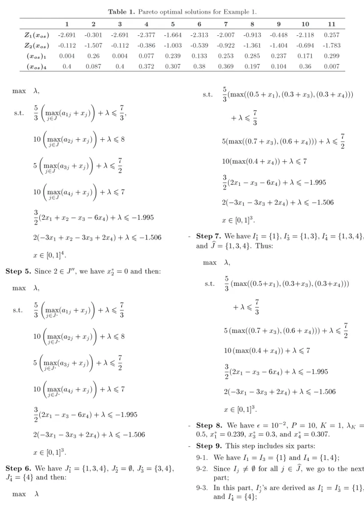
By the optimization toolbox of Matlab software and \gamultiobj" solver, which uses the Genetic algorithm for solving multi-objective problems, 11 Pareto optimal solutions have been computed for the problem of this step and they are presented in Table 1, where (xos)2 = 0 and (xos)3 = 0:3 for all

Pareto optimal solutions. Assume the DM has chosen xos = (0:239; 0; 0:3; 0:307). Therefore, Z1(xos) =

1:664 and Z2(xos) = 1:003.

- Step 4. We have D1 = 5₃, D2 = 10, D3 = 5, D4 =

10, D1

0 = 32, D20 = 2, B1 = 7₃, B2 = 8, B3 = 7₂,

B4 = 7, z1 = 1:997, z2 = 1:253, B01 = 1:995,

and B2

0 = 1:506. Thus, the problem is converted to

Table 1. Pareto optimal solutions for Example 1.

1 2 3 4 5 6 7 8 9 10 11

Z1(xos) -2.691 -0.301 -2.691 -2.377 -1.664 -2.313 -2.007 -0.913 -0.448 -2.118 0.257

Z2(xos) -0.112 -1.507 -0.112 -0.386 -1.003 -0.539 -0.922 -1.361 -1.404 -0.694 -1.783

(xos)1 0.004 0.26 0.004 0.077 0.239 0.133 0.253 0.285 0.237 0.171 0.299

(xos)4 0.4 0.087 0.4 0.372 0.307 0.38 0.369 0.197 0.104 0.36 0.007

max ;

s.t. 5₃

max

j2J(a1j+ xj)

+ 6 7₃;

10

max

j2J(a2j+ xj)

+ 6 8

5

max

j2J(a3j+ xj)

+ 6 7₂

10

max

j2J(a4j+ xj)

+ 6 7

3

2(2x1+ x2 x3 6x4) + 6 1:995 2( 3x1+ x2 3x3+ 2x4) + 6 1:506

x 2 [0; 1]4_:

- Step 5. Since 2 2 J00_{, we have x}

2= 0 and then:

max ;

s.t. 5₃

max

j2J(a1j+ xj)

+ 6 7₃

10

max

j2J(a2j+ xj)

+ 6 8

5

max

j2J(a3j+ xj)

+ 6 7₂

10

max

j2J(a4j+ xj)

+ 6 7

3

2(2x1 x3 6x4) + 6 1:995 2( 3x1 3x3+ 2x4) + 6 1:506

x 2 [0; 1]3_:

- Step 6. We have J

1= f1; 3; 4g, J2 = ;, J3= f3; 4g,

J

4= f4g and then:

max

s.t. 5₃(max((0:5 + x1); (0:3 + x3); (0:3 + x4)))

+ 6 7₃

5(max((0:7 + x3); (0:6 + x4))) + 6 7₂

10(max(0:4 + x4)) + 6 7

3

2(2x1 x3 6x4) + 6 1:995 2( 3x1 3x3+ 2x4) + 6 1:506

x 2 [0; 1]3_:

- Step 7. We have I

1= f1g, I3 = f1; 3g, I4= f1; 3; 4g,

and bJ = f1; 3; 4g. Thus: max ;

s.t. 5₃(max((0:5+x1); (0:3+x3); (0:3+x4)))

+ 6 7₃

5 (max((0:7 + x3); (0:6 + x4))) + 6 7₂

10 (max(0:4 + x4)) + 6 7

3

2(2x1 x3 6x4) + 6 1:995 2( 3x1 3x3+ 2x4) + 6 1:506

x 2 [0; 1]3_:

- Step 8. We have = 10 2_{, P = 10, K = 1,} K =

0:5, x

1= 0:239, x3= 0:3, and x4= 0:307.

- Step 9. This step includes six parts:

9-1. We have I1= I3= f1g and I4= f1; 4g;

9-2. Since Ij 6= ; for all j 2 bJ, we go to the next

part;

9-3. In this part, I

j's are derived as I1 = I3 = f1g,

and I 4= f4g;

9-4 Since I

1TI3 6= ;, the problem of Step 7 should

be converted to the form Relation (18). We have I= f1g, J10 = f1; 3g, J= f4g and thus:

max ;

s.t. 5₃(0:5 + x1) + 67₃

5

3(0:3 + x3) + 6 7 3 10(0:4 + x4) + 6 7

3

2(2x1 x3 6x4) + 6 1:995 2( 3x1 3x3+ 2x4) + 6 1:506

x 2 [0; 1]3_:

9-5. Solving the problem in step 9-4, we have x1=

0:0, x3= 0:595, x4= 0:215, and = 0:841;

9-6. Since < 1 by considering K = 2 and K=

0:841, we repeat Step 9.

In the second repetition of Step 9, we have:

9-1. I1= I3= f1g and I4= f1; 4g;

9-2. Ij 6= ; for all j 2 bJ and thus, we go to the next

part;

9-3. We have I

1= I3= f1g and I4 = f4g;

9-4. Since I = f1g, J10 = f1; 3g and J = f4g, the

problem in this part is similar to the problem in step 9-4 in the previous repetition;

9-5. We have x1= 0:0, x3 = 0:595, x4= 0:215, and

= 0:841.

As it is seen that K = K 1 and hence, we should

break this step.

- Step 10. We have x

1= 0:0, x3= 0:595, x4= 0:215,

and _{= 0:841.}

- Step 11. Z1(x) = 1:885 and Z2(x) = 1:355,

which are the optimal values of the problem.

- Step 12. End.

Hence, in this example, the fuzzy solution is (0; 0; 0:595; 0:215) and its values in objective functions are -1.885 and -1.355, respectively. If the DM is not satised with this fuzzy solution, he/she should accept more perturbation in constraints or choose another solution in Step 3 of Algorithm 1.

5. Conclusion

We have used Max-Arithmetic mean composition in a multi-objective optimization problem subject to a system of fuzzy relational inequalities in which ordinary

inequalities have been replaced by fuzzy inequalities to benet from the advantages of this composition and obtain more realistic solutions. Assigning linear membership functions to the inequalities and objective functions using one selected solution of the same multi-objective optimization problem with ordinary inequal-ities and employing Bellman-Zadeh decision, we have converted the multi-objective optimization problem in the presence of fuzzy inequalities in its constraints into a new simpler one in order to use infeasible points to obtain better solutions. Afterwards, we have diminished the dimension of the problem and proposed an algorithm to generate the optimal solution. If the algorithm yields a solution similar to the one which is obtained using only the feasible points, then the decision maker should accept more perturbation on the constraints. Also, in the case that the decision maker is not satised with the obtained solution by the algorithm, he/she should accept more perturbation on the constraints as well or choose another solution to the ordinary multi-objective optimization problem. This process should be continued until the desired solution of the decision maker is achieved. For future studies, it seems useful to employ other kinds of membership functions as they have been mentioned in Remark 1.

References

1. Khorram, E. and Zarei, H. \Multi-objective optimiza-tion problems with fuzzy relaoptimiza-tion equaoptimiza-tion constraints regarding max-average composition", Math. Comput. Modeling, 49, pp. 856-867 (2009).

2. Yang, S.J. \An algorithm for minimizing a linear objec-tive function subject to the fuzzy relation inequalities with addition-min composition", Fuzzy Sets Syst., 255, pp. 41-51 (2014).

3. Zhou, X.G., Yang, X.P. and Cao, B.Y. \Posynomial geometric programming problem subject to max-min fuzzy relation equations", Inf. Sci., 328, pp. 15-25 (2016).

4. Kouchakinejad, F., Khorram, E. and Mashinchi, M. \Fuzzy optimization of linear objective function sub-ject to max-average relational inequality constraints", J. Intell. Fuzzy Syst., 29, pp. 635-645 (2015).

5. Shivanian, E., Khorram, E. and Ghodousian, A. \Optimization of linear objective function subject to fuzzy relation inequalities constraints with max-average composition", Iran. J. Fuzzy Syst., 4, pp. 15-29 (2007).

6. Abbasi Molai, A. \Resolution of a system of the max-product fuzzy relational equations using LU-factorization", Inf. Sci., 234, pp. 86-96 (2013).

7. Hassanzadeh, R., Khorram, E., Mahdavi, I. and Amiri, N.M. \A genetic algorithm for optimization

problems with fuzzy relation constraints using max-product composition", Appl. Soft Comp., 11, pp. 551-560 (2011).

8. Khorram, E., Ezzati, R. and Valizadeh, Z. \Linear fractional multi-objective optimization problems sub-ject to fuzzy relational equations with a continuous Archimedean triangular norm", Inf. Sci., 267, pp. 225-239 (2014).

9. Guu, S.M., Wu, Y.K. and Lee, E.S. \Multi-objective optimization with a max-t-norm fuzzy relational equa-tion constraint", Comput. Math. Appl., 61, pp. 1559-1566 (2011).

10. Zimmermann, H.J., Fuzzy Set Theory and Its Applica-tion, Kluwer Academic Publishers, Boston, Dordrecht, London (1991).

11. Kouchakinejad, F., Khorram, E. and Mashinchi, M. \Solving multi-objective optimization problems with fuzzy max-arithmetic mean relational inequality con-straints", Proceedings of 1th Conf. on Research in Advanced Sciences of Mathematics (On a CD-Rom), Urmia, Iran, Paper No. RAMS338 (2015).

12. Sakawa, M., Fuzzy Sets and Interactive Multi-Objective Optimization, Plenum Press, New York, (1993).

13. Ghodousian, A. and Khorram, E. \Fuzzy linear opti-mization in the presence of the fuzzy relation inequality constraints with max-min composition", Inf. Sci., 178, pp. 501-519 (2008).

14. Bellman, R.E. and Zadeh, L.A. \Decision-making in fuzzy environment", Manag. Sci., 17, pp. 141-164 (1970).

15. Mitchell, M., An Introduction to Genetic Algorithms, 5th Edn., MIT Press, Cambridge, MA (1999).

Biographies

Fateme Kouchakinejad is currently PhD candidate in Applied Mathematics at Graduate University of Advanced Technology in Kerman, Iran. Her research interests include fuzzy optimization, fuzzy relational equations/inequalities, and fuzzy bags and aggregation functions.

Mashaallah Mashinchi was born in Kerman, Iran. He received his BSc degree in 1976 and MSc degree in 1978, both in Statistics from Ferdowsi University and Shiraz University, Iran, respectively, and his PhD degree in 1987 in Mathematics from Waseda University, Japan. He is now a Professor in the Department of Statistics at Shahid Bahonar University of Kerman, Kerman, Iran. His current interest is in fuzzy math-ematics, especially statistics, decision making, and algebraic systems.

Esmaile Khorram obtained his PhD degree in Ap-plied Mathematics from Bradford University, England, in 1989. He is currently professor in Optimization and Statistics at Amirkabir University of Technology, Tehran, Iran.