Teaching Learning Based Optimization for Different ‎Economic Dispatch Problems

(1)

Sharif University of Technology

Scientia Iranica

Transactions D: Computer Science & Engineering and Electrical Engineering www.scientiairanica.com

Teaching-learning-based optimization for dierent

economic dispatch problems

K. Bhattacharjee

a

_{, A. Bhattacharya}

b;

_{and S. Halder nee Dey}

c

a. Department of Electrical Engineering, Dr. B.C. Roy Engineering College, Durgapur, West Bengal, 713206, India. b. Department of Electrical Engineering, National Institute of Technology, Agartala, Tripra, 799055, India.

c. Department of Electrical Engineering, Jadavpur University, Kolkata, West Bengal, 700 032, India. Received 1 November 2012; received in revised form 14 April 2013; accepted 23 November 2013

KEYWORDS Economic load dispatch;

Prohibited operating zone;

Ramp rate limits; Teaching-learning optimization; Valve-point loading.

Abstract. This paper presents a Teaching-Learning-Based Algorithm (TLBO) to solve Economic Load Dispatch (ELD) problems involving dierent linear and non-linear constraints. The problem formulation also considers non-convex objective functions including the eect of valve-point loading and the multi-fuel option of large-scale thermal plants. Many diculties, such as multimodality, dimensionality and dierentiability, are associated with the optimization of large scale non-linear constraint based non-convex economic load dispatch problems. TLBO is a population-based technique which implements a group of solutions to proceed to the optimum solution. TLBO uses two dierent phases; `Teacher Phase' and `Learner Phase', and uses the mean value of the population to update the solution. Unlike other optimization techniques, TLBO does not require any parameter to be tuned, thus, making its implementation simpler. TLBO uses the best solution of the iteration to change the existing solution in the population, thereby increasing the convergence rate. In the present paper, Teaching-Learning-Based Optimization (TLBO) is applied to solve such types of complicated problems eciently and eectively, in order to achieve a superior quality solution in a computationally ecient way. Simulation results show that the proposed approach outperforms several existing optimization techniques. Results also proved the robustness of the proposed methodology.

c

1. Introduction

Economic load dispatch is the process of allocating gen-eration among the available generating units, consider-ing the most ecient, reliable and low cost operation of a power system, providing that load demand and other operational constraints are satised. Its main aim is to minimize the total cost of generations, while satisfying the operational constraints of the available thermal power generation resources. Initially, traditional tech-*. Corresponding author. Tel.: +91 9474188660

E-mail addresses: kunti [email protected] (K. Bhattacharjee); ani [email protected] (A. Bhattacharya); [email protected] (S. Halder nee Dey)

niques [1] were applied to solve ELD problems. The linear programming method [2] is fast and reliable, but also has some drawbacks, and classical optimization techniques are excellent for uni-modal and continuous functions. In these methods, the essential assumption is that the incremental costs and emission curves of the generating units are monotonically increasing or piece-wise linear. A practical ELD problem sometimes takes the eect of valve-point loading, ramp-rate limits, prohibited operating zones, multi-fuel options etc. into consideration. Due to all these practical eects, the resulting ELD problems have become totally non-convex optimization problems. Therefore, in some cases, these methods converge to a locally, not globally, optimal solution. The Dynamic Programming (DP)

(2)

approach was proposed by Wood and Wollenberg [3] to solve ELD problems. It imposes no restrictions on the characteristics of the generating units. However, it suers from the curse of dimensionality and also increases execution time with the increase in system size.

Several attempts have been made to solve ELD problems using various soft computing techniques, such as Genetic Algorithms (GA) [4-5], Particle Swarm Optimization (PSO) [6], Ant Colony Optimiza-tion (ACO) [7], EvoluOptimiza-tionary Programming (EP) [8], Simulated Annealing (SA) [9], Dierential Evolution (DE) [10], Articial Immune System (AIS) [11], Bacte-rial Foraging Algorithm (BFA) [12], and Biogeography-Based Optimization (BBO) [13] etc. The above-mentioned techniques have proven to be very fast and reasonably near a global optimal solution in solving nonlinear ELD problems, without any restriction on the shape of the cost curves. Recently, dierent hybridizations and modications of GA, EP, PSO, DE and BBO have been adopted to solve dierent types of ELD problems, such as Improved GA with Multiplier Updating (IGA-MU) [14], hybrid Genetic Algorithm (GA)-Pattern Search (PS)-Sequential Quadratic Pro-gramming (SQP) (GA-PS-SQP) [15], Improved Fast Evolutionary Programming (IFEP) [16], New PSO with Local Random Search (NPSO LRS) [17], Adap-tive PSO (APSO) [18], Self-Organizing Hierarchical-PSO (SOH-Hierarchical-PSO) [19], Improved Coordinated Aggre-gation based PSO (ICA-PSO) [20], improved PSO [21], Combined Particle Swarm Optimization with Real-Valued Mutation (CBPSO-RVM) [22], DE with gen-eration of chaos sequences and Sequential Quadratic Programming (DEC-SQP) [23], Variable Scaling Hy-brid Dierential Evolution (VSHDE) [24], hyHy-brid Dif-ferential Evolution (DE) [25], Bacterial Foraging with Nelder-Mead algorithm (BF-NM) [26], and hybrid Dierential Evolution with Biogeography-Based Opti-mization (DE/BBO) [27] etc.

Evolutionary algorithms, swarm intelligence and bacterial foraging all are population-based bio-inspired algorithms. However, the common disadvantages of these algorithms are their complicated computations, needing many parameters, and, therefore, for beginners they are dicult to understand. Moreover, all the nature-inspired algorithms, such as GA, EP, PSO, ACO, DE, BFA, AIS, BBO etc., require tuning of al-gorithm parameters for them to work properly. Proper selection of parameters is essential for the searching of the optimum solution by these algorithms, and a change in the algorithm parameters changes their eectiveness. To avoid this diculty, an optimiza-tion method, Teaching-Learning-Based Optimizaoptimiza-tion (TLBO), a parameter free algorithm, is implemented in this paper to solve complex ELD problems.

Teaching-Learning-Based Optimization (TLBO)

was proposed by Rao et al. in 2011 [28]. This method works like the eect of the inuence of a teacher on learners. Like other nature-inspired algorithms, TLBO is also a population-based method, which uses a population of solutions to proceed to the global solution. For TLBO, the population is considered as a group or a class of learners. The process when using TLBO is divided into two parts. The rst part consists of the `Teacher Phase' and the second part consists of the `Learner Phase'. The `Teacher Phase' means learning from the teacher and the `Learner Phase' means learning through interaction between learners. The teacher is generally considered a highly learned person who shares his or her knowledge with the learners. The quality of a teacher aects the outcome of the learners. It is obvious that a good teacher trains learners such that they can have better results in terms of their marks or grades. Moreover, learners also learn from interaction between themselves, which also helps in their results. Like several other soft computing tech-niques, TLBO is also a population-based technique, which implements a group of solutions to proceed to the optimum solution. Many optimization methods require algorithm parameters that aect techniques, TLBO does not require any algorithm parameters to be tuned, thus making the implementation of TLBO simpler. TLBO uses the best solution of the iteration to change the existing solution in the population, thereby increasing the convergence rate. TLBO uses the mean value of the population to update the solution and, therefore, implements greediness to accept a good solution. It has been already observed that the performance of TLBO is quite satisfactory when applied to solving continuous benchmark optimization problems [28].

The improved performance of TLBO in solving continuous benchmark optimization problems has mo-tivated the present authors to implement this newly developed algorithm to solve dierent complex ELD problems. This paper considers four types of ELD problem, namely (i) ELD with quadratic cost func-tion, ramp rate limit, prohibited operating zone and transmission loss: 15 generators system, (ii) ELD with quadratic cost function without transmission loss: 38 generators system, (iii) ELD with valve-point eects, ramp rate limit, prohibited operating zone: 140 generators system, (iv) ELD having multiple fuels and valve-point eects: 160 generators sys-tem.

Section 2 of the paper provides mathematical for-mulation of dierent types of ELD problems. Section 3 describes the proposed TLBO algorithm, along with a short description of the algorithm used in these test systems. Simulation studies are presented and discussed in Section 4 and the conclusion is drawn in Section 5.

(3)

2. Mathematical modeling of the ELD problem The ELD may be formulated as both convex and non-convex nonlinear constrained optimization problems. Four dierent types of ELD problem have been for-mulated and solved using the TLBO approach. These are presented below.

2.1. ELD with quadratic cost function, ramp rate limit, prohibited operating zone and transmission loss

The overall objective function, FT, of the ELD problem

may be written as: FT = min

N

X

i=1

Fi(Pi)

= min

N

X

i=1

(ai+ biPi+ ciPi2); (1)

where Fi(Pi) is the cost function of the ith generator

and is usually expressed as a quadratic polynomial; N is the number of committed generators; ai, bi and ci

are the cost coecients of the ith generator; Pi is the

power output of the ith generator. The ELD problem consists in minimizing the FT subject to the following

constraints:

1) Real power balance constraint:

N

X

i=1

Pi (PD+ PL) = 0; (2)

where PDis the total system active power demand,

and PL is the total transmission loss. Calculation

of PL using the B-coecients matrix is expressed

as: PL=

N X i=1 N X j=1

PiBijPj+ N

X

i=1

B0iPi+ B00: (3)

2) The generating capacity constraint: The power must be generated by each generator within their lower limit, Pmin

i , and upper limit, Pimax, so that:

Pmin

i Pi Pimax; (4)

where Pmin

i and Pimax are the minimum and the

maximum power outputs of the ith unit.

3) Ramp rate limit constraint: The power, Pi,

gener-ated by the ith generator at certain intervals neither should exceed that of the previous interval, Pio,

by more than a certain amount, URi, the up-ramp

limit, nor should it be less than that of the previous interval by more than some amount, DRi, the

down-ramp limit of the generator. These give rise to the following constraints:

As generation increases:

Pi Pio URi: (5)

As generation decreases:

Pio Pi DRi; (6)

max Pmin

i ; Pi0 DRi(Pimax; Pi0+URi) : (7)

4) Prohibited operating zone: Mathematically, the feasible operating zones of a unit can be described as follows:

Pmin

i Pi Pi;1l ;

Pu

i;j 1 Pi Pi;jl ; j = 2; 3; :::; ni;

Pu

i;ni Pi P

max

i ; (8)

where j represents the number of prohibited operat-ing zones of unit i. Pu

i;jis the upper limit and Pi;jl is

the lower limit of the jth prohibited operating zone of the ith unit. The total number of prohibited operating zones of the ith unit is nj.

2.2. ELD with quadratic cost function

In this type of ELD problem, the overall objective function is the same as mentioned in Eq. (1). Here, the objective function, FT, is to be minimized, subject

to the constraints of Eqs. (2) and (4). Here, PL is

zero.

2.3. ELD with valve-point eects, ramp rate limit, prohibited operating zone

The fuel cost function, FT, in the ELD problem with

valve point loading changes the simple cost function in Eq. (1). It becomes more complex and is represented below:

FT = N

X

i=1

Fi(Pi)

! =

_XN i=1

ai+ biPi+ ciPi2

+ei sin

fi (Pimin Pi)

; (9)

where ei and fi, the coecients of the ith generator,

reect the valve-point eects. The objective function in Eq. (9) is to be minimized, subject to the same set of constraints given in Eqs. (4), (7) and (8).

2.4. ELD with non-smooth cost functions with multiple fuels and valve-point eects For a power system with N generators and nF fuel

options for each unit, the cost function of the generator with valve-point loading is expressed as:

(4)

Fi(Pi) =aip+ bipPi+ cipPi2

+eip sin

fip (Pipmin Pip); (10)

if Pmin

ip Pi Pipmax for fuel option p;

p = 1; 2; :::; nF;

where Pmin

ip and Pipmaxare the minimum and maximum

power generation limits of the ith generator with fuel option, p, respectively; aip, bip, cip, eip and fip are

the fuel-cost coecients of the ith generator for fuel option p.

Considering N number of generators, the above-mentioned objective function is to be minimized sub-ject to the constraints of Eqs. (2) and (4), without considering transmission loss. Therefore, the PL term

in Eq. (2) becomes zero.

2.5. Calculation for slack generator

Let N committed generating units deliver their power output, subject to the power balance constraint in Eq. (2) and the respective capacity constraints of Eqs. (4) and/or (7), and (8). Assuming the power loadings of the rst (N 1) generators are known, the power level of the Nth generator (called the Slack Generator) is given by:

2.5.1 Without transmission loss: PN = PD

(N 1)_X i=1

Pi: (11)

2.5.2 With transmission loss: PN = PD+ PL

(N 1)_X i=1

Pi: (12)

Using Eqs. (3) and (12), the modied form of the equation is:

BNNPN2 + PN

2N 1X

i=1

BNiPi+ N 1_X

i=1

BON 1

+

P D +N 1X

i=1 N 1_X

j=1

PiPijPj

+

N 1_X i=1

BOiPi N 1_X

i=1

Pi+ BOO

= 0:

(13) The solution procedure of Eq. (13) to calculate slack generator output, PN, is the same as mentioned

in [19]. To avoid repetition, it is not presented here.

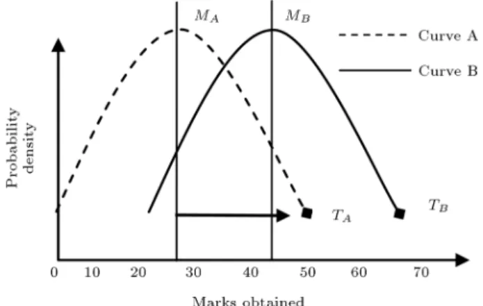
Figure 1. Marks distribution by learners taught by T1 and T2.

3. Teaching-learning-based algorithm

This section presents an interesting new optimization algorithm called Teaching-Learning-Based Optimiza-tion (TLBO), which has been recently proposed in [28]. The TLBO method works on the philosophy of the eect of manipulation of a teacher on the output of learners in a class, and, consequently, learning by interaction between class members, which helps in their grades. Therefore, the TLBO method works on the philosophy of teaching and learning.

Consider two dierent teachers, T1and T2,

teach-ing a topic to the same merit level learners in two dierent classes. The distribution of marks obtained by the learners for these two varying classes is evaluated by the teachers and is illustrated in Figure 1. Curves 1 and 2 represent the evaluated marks obtained by the learners taught by teacher T1and T2, respectively.

Nor-mal distribution for the goal achieved by the learners is dened as:

f(x) = 1 p2e

(x )2

2 ; (14)

where 2 _{is the variance, is the mean, and x is}

any value of whichever normal distribution function is required. Comparing the mean value of Curves 1 and 2 of Figure 1, it is seen that the learners from Curve 2 get better results than the learners from Curve 1. So, it can be said that teacher T2 is better than teacher

T1 in terms of teaching. Learners also learn from

interaction between themselves, which promotes their results.

Figure 2 shows a model for the marks obtained by the learners in a class having mean MAin Curve A.

Teachers are considered the most intelligent members of society and, therefore, the best learner is considered to be the teacher here. This is shown by TA in

Figure 2. The teacher tries to spread knowledge among the learners, which, in turn, increases the knowledge level of the whole class and help learners to get good marks or grades. Teacher TA puts maximum eort

(5)

Figure 2. Distribution of score for learners.

into teaching his or her students and tries to move class mean from MA towards a new mean, MB, by

means of increasing the learners' knowledge level. At that stage, the learners require a new teacher, TB, of

superior quality than themselves, which is shown by Curve B in Figure 2.

TLBO is also a population-based algorithm, whose population is described as a class of learners. In any nature-inspired based optimization algorithms, the population consists of dierent design variables. In TLBO, dierent design variables are the dierent subjects oered to the learners, and the learners' out-come corresponds to the `tness function'. The teacher is considered the best solution obtained so far. The process of TLBO is divided into two parts. `Teacher Phase' and `Learner Phase'. The `Teacher Phase' means learning from the teacher and the `Learner Phase' means learning through interaction between learners. These two parts of TLBO are described below.

3.1. Teacher phase

A good teacher always tries to improve the quality of learners in terms of knowledge, i.e. a teacher tries to increase the mean value of the class from MA to

MB, as seen in Figure 2. But, in real practice, this is

not possible and a teacher can only move the average quality of a class up to some limit, depending on the quality of the class.

Let Mk be the mean and Tk be the teacher at

any iteration, k. Tk tries to move mean Mk towards

its own level. The solution is updated according to the dierence between the existing and the new mean. It is given by:

Xdi= rand()x(Tk RtMk); (15)

where, rand() is a random number in the range [0,1]; the value of Rt can be either 1 or 2, which can be

decided randomly with equal probability.

This dierence modies the existing solution ac-cording to the following expression:

Xnew= Xold+ Xdi: (16)

3.2. Learner phase

In the learner phase, the learners increase their knowl-edge by two dierent methods. The rst is through input from the teacher and the other through some interaction between themselves. A learner interacts with other randomly selected learners by participation in formal communication, group discussion and pre-sentations. By interaction, a learner learns something new if the other learners have more knowledge than the corresponding learner [28]. In order to design the mathematical model, two learners, Xi and Xj, are

randomly chosen, where i 6= j. Objective functions for the learners, Xi and Xj, are evaluated. The achieved

objective functions of Xi and Xj are compared. If

the achieved objective function of Xi is less than the

achieved objective function of Xj, then:

Xnew= Xold+ rand()x(Xi Xj): (17)

Otherwise:

Xnew= Xold+ rand()x(Xj Xi): (18)

If the new solution is better than the existing one, then it is accepted. The pseudo codes and ow chart for all steps are available in [28].

3.3. Sequential steps of TLBO algorithm There are two stages in TLBO: teacher phase and learner phase. All the steps are mentioned below: 1) At the initialization stage, read in the initial

num-ber of learners (PopSize) (equivalent to population size of many heuristic algorithms); maximum it-eration number (Itermax). Specify the number of

design variables (D), in this case, assigned as the number of subjects oered. Mention the lower and upper limits of design variables.

2) Generate the learner matrix (Xij) randomly,

ac-cording to population size, number of design vari-ables and limits of the varivari-ables (where i = 1; 2:::. PopSize, and j = 1; 2; :::D and total matrix size is PopSize D).

3) Determine objective function values for each learner set. The size of the objective function matrix is, therefore PopSizeD. The minimum value to come out of these objective function values is the local optimum value, and the corresponding value of Xij

is set as the teacher (Xteacher). So, Xteacher= Tkin

Eq. (15).

4) Calculate the mean value of each design variable column-wise. So, the size of the mean value is 1D, and is used in Eq. (15) as Mk.

5) Modify each learner by Eqs. (15) and (16). The value of Rtis randomly selected as 1 or 2. Calculate

(6)

the objective function values for each modied learner. If the new value of the objective function of any learner is better than the previous one, then accept a new learner and replace the corresponding old one. Otherwise, keep the old learner without any modication.

6) Learner phase: Learners increase their knowledge with the help of mutual interaction. For each learner Xi(i = 1; 2; :::::D), arbitrarily choose any

learner, Xj, from the learner matrix. Compare

the objective function corresponding to Xi and

Xj. If the value of the objective function of Xi is

lower than the objective function value of Xj, then

modify the ith learner using Eq. (17), otherwise, modify the ith learner using Eq. (18).

7) If the maximum number of iterations is reached or the specied accuracy level is achieved, terminate the iterative process, otherwise, go to step 3 for continuation. Interested readers may refer to [28] which contains detailed steps of the TLBO Algo-rithm.

3.4. TLBO algorithm for economic load dispatch problem

In this subsection, the procedure to implement the TLBO algorithm for solving ELD problems has been described. This algorithm is also used to deal with the equality and inequality constraints of ELD problems. The sequential steps of the TLBO algorithm applied to solve the ELD problem are:

1) Representation of the learner matrix, X: Since the assessment variables for the ELD problem are the real power output of the generators, they are together used to represent the individual learner. Each individual element of a learner is the subject studied by the corresponding learner, and it is same as the real power outputs of the generators in ELD. For initializations, choose the number of generator units, m, as a design variable, D. The total number of the learner structure is population size, which is denoted as `PopSize'.

The complete learner matrix is represented in the form of the following matrix:

X = Xi= [X1; X2; X3; :::; XPopSize] (19)

where i = 1; 2; :::; Popsize.

In the case of the ELD problem, each learner is presented as:

Xi= [Xi1; Xi2; :::; Xim] = [P gij]

= [P gi1; P gi2; :::; P gim];

where, j = 1; 2; :::; m: Each learner is one of the possible solutions for the ELD problem. The

element, Xij, of Xi is the jth position component

of learner, i.

2) Initialization of the learner: Each individual ele-ment of the learner matrix (X), i.e. each eleele-ment of a given learner, is initialized randomly within the eective real power operating limits. The initial-ization is based on Eq. (4) for generators without ramp rate limits, on Eqs. (4) and (7) for generators with ramp rate limits and on Eqs. (4), (7) and (8) for generators with ramp rate limits, prohibited operating zone.

3) Evaluation of objective functions: In the case of ELD problems, the objective function of each learner is represented by the total fuel cost of generation for all the generators of that given learner. It is calculated using Eq. (1) for the system having quadratic fuel cost characteristics, Eq. (9) for the system having valve-point eects, and Eq. (10) for the system having multi-fuel type fuel cost characteristics.

Now, the steps of the algorithm to solve ELD problems are given below:

- Step 1. For initialization, choose the number of generator units, m, i.e. number of design variables, D, and number of learners, PopSize. Specify the maximum and minimum capacity of each generator, the power demand, the B-coecient matrix for calculation of transmission loss and other input data. Set the maximum number of iterations, Itermax.

- Step 2. Each learner of the X matrix should satisfy the equality constraint of Eq. (2) using the concept of slack generator, as mentioned in Section 2.5. - Step 3. Calculate the objective function value for

each learner following the procedure mentioned in \Evaluation of objective functions".

- Step 4. Based on objective function values, identify the elite learner, which is assigned as the teacher of the learner matrix. Here, the elite term is used to indicate the learner that gives the best fuel cost. The elite learner is taken as Tk in Eq. (15).

- Step 5. From the learner matrix (X), calculate the mean value of each design variable, i.e. the mean value of the individual generator power output column wise. The mean value is assigned as Mk in

Eq. (15).

- Step 6. Modify each learner, i.e. the power output of the generators, using Eqs. (15) and (16). Verify the feasibility of each newly generated learner of the modied X matrix. Individual elements of each modied learner must satisfy the generator operating limit constraint of Eq. (4). If any element of a learner violates either upper or lower operating limits, then

(7)

x the values of those elements of the corresponding learner at the limit reached by them. Again, satisfy the constraint of Eq. (2) using the concept of slack generator, as presented in Section 2.5 (PL = 0 in

Eq. (12) if loss is not considered). If the output of the slack generator does not meet generator operating limit constraint, as in Eq. (4), or some generators do not satisfy the prohibited operating zone or ramp rate limit constraints, where applicable, then reject that new learner and reapply Step 6 on the old one, until all constraints are satised.

- Step 7. Calculate the values of the objective function of each modied learner of the learner matrix. If the new value of the objective function of any learner is better than the previous one, then accept the new learner and replace the corresponding old one. Otherwise, keep the old learner without any modication.

- Step 8. For each learner, Xi(i = 1; 2; ::::; D),

arbitrarily choose any learner, Xj, from the learner

matrix. Compare the objective function correspond-ing to Xi and Xj. If the value of the objective

function of Xi is lower than the objective function

value of Xj, then modify the ith learner using

Eq. (17). Otherwise, modify the ith learner using Eq. (18).

- Step 9. Individual elements of each modied learner must satisfy their generator constraints. If any element of a modied learner violates either upper or lower operating limits, then x the values of those elements of the corresponding learner at the limit reached by them. Again, satisfy the constraint of Eq. (2) using the concept of the slack generator, as presented in Section 2.5 (PL = 0 in Eq. (12) if

loss is not considered). If the output of the slack generator does not meet the generator operating limit constraint, as in Eq. (4), or some generators do not satisfy the prohibited operating zone or ramp rate limit constraints, where applicable, reject that modied learner and reapply Step 8 on the old one, until all the constraints are satised.

- Step 10. As individual learners of the learner matrix change, the values of their objective function also change. Calculate the objective function of each newly generated learner. If the new value of the objective function of a given learner is better than its previous value, then accept the new learner and replace the corresponding old one. Otherwise, keep the old learner without any modication.

- Step 11. If the maximum number of iterations is reached or specied accuracy level is achieved, terminate the iterative process. Otherwise, go to Step 4 for continuation.

4. Examples and simulation result

The proposed TLBO algorithm has been applied to solve ELD problems in four dierent test cases, and its performance has been compared to several other optimization techniques, like GA [7], DE/BBO [7,27], and PSO [7,21] etc., for verifying its feasibility. The necessary codes have been written in MATLAB-7 language and executed on a 2.0-GHz Intel Pentium (R) Dual Core personal computer with 1-GB RAM. 4.1. Description of the test systems

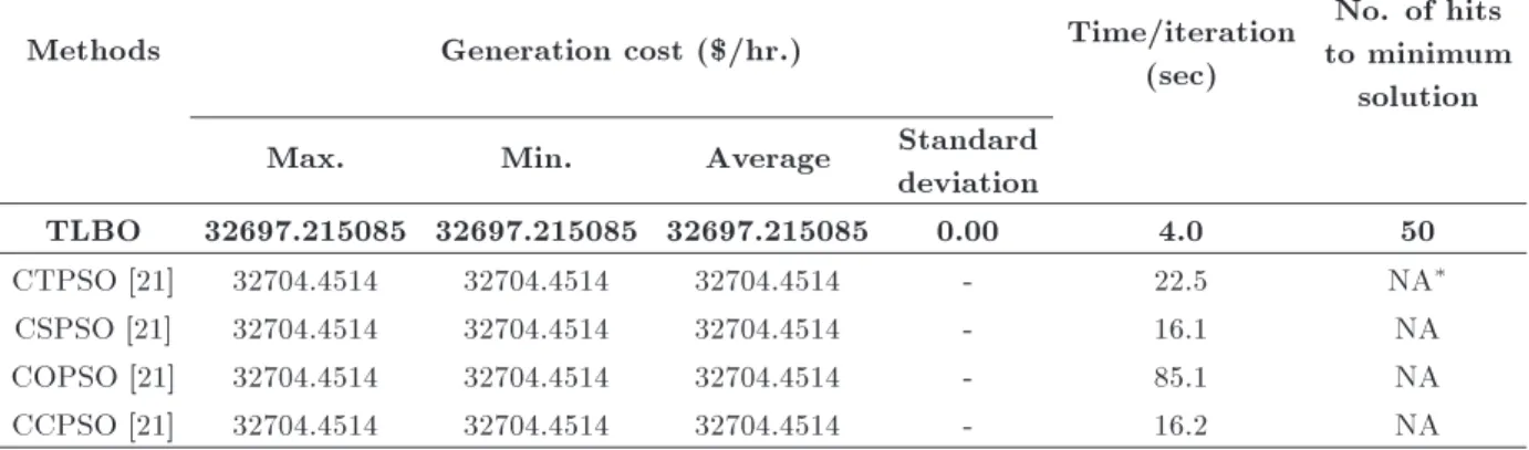
Test system 1: In this example, 15 generating units with ramp rate limit and prohibited zone constraints have been considered. Transmission loss has been included in the problem. Power demand is 2630 MW and system data have been taken from [7]. Results obtained from the proposed TLBO, PSO [7], dierent versions of PSO [21] and other method, have been presented here, and their best solutions are shown in Table 1. The convergence characteristics of the 15-generator system in the case of TLBO are shown in Figure 3. Minimum, average and maximum fuel costs obtained by TLBO and dierent versions of PSO [21], over 50 trials, are presented in Table 2.

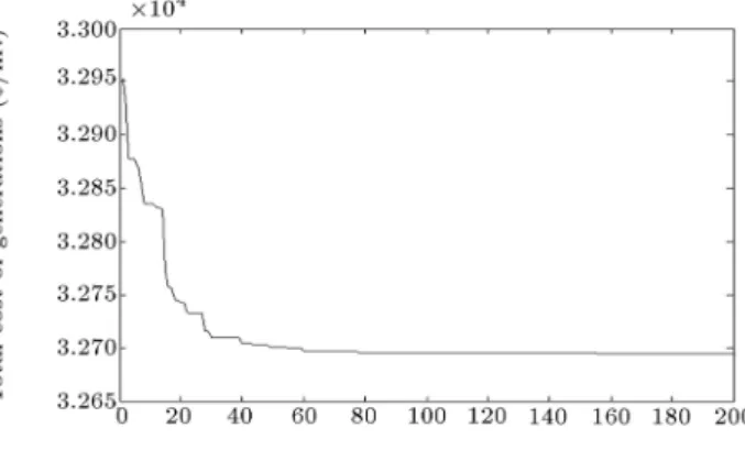
Test system 2: A 38-generator system with quadratic fuel cost characteristics is used here. The input data are taken from [29]. The load demand is 6000 MW. Transmission loss has not been consid-ered here. The result obtained using the proposed TLBO method has been compared with BBO [27], DE/BBO [27], PSO-TVAC [27] and New-PSO [27], whose best solutions are shown in Table 3. A con-vergence characteristic of the 38-generator system in the case of TLBO are shown in Figure 4. Minimum, average and maximum fuel costs obtained by TLBO over 50 trials are shown in Table 4.

Test system 3: A 140-generator system having ramp rate limit and prohibited zone constraints is considered. The eect of valve-point loading has

Figure 3. Convergence characteristic of 15-generator systems, obtained by TLBO.

(8)

Table 1. Best power output for 15-generator systems (PD= 2630 MW).

Unit TLBO GA [7] PSO [7] CTPSO [21] CSPSO [21] COPSO [21] CCPSO [21] 1 455.000000 415.3108 439.1162 455.0000 455.0000 455.0000 455.0000 2 380.000000 359.7206 407.9727 380.0000 380.0000 380.0000 380.0000 3 130.000000 104.4250 119.6324 130.0000 130.0000 130.0000 130.0000 4 130.000000 74.9853 129.9925 130.0000 130.0000 130.0000 130.0000 5 170.000000 380.2844 151.0681 170.0000 170.0000 170.0000 170.0000 6 460.00000 426.7902 459.9978 460.0000 460.0000 460.0000 460.0000 7 430.000000 341.3164 425.5601 430.0000 430.0000 430.0000 430.0000 8 73.081166 124.7867 98.5699 71.7430 71.7408 71.7427 71.7526 9 51.646599 133.1445 113.4936 58.9186 58.9207 58.9189 58.9090 10 160.000000 89.2567 101.1142 160.0000 160.0000 160.0000 160.0000 11 80.000000 60.0572 33.9116 80.0000 80.0000 80.0000 80.0000 12 80.000000 49.9998 79.9583 80.0000 80.0000 80.0000 80.0000 13 26.577183 38.7713 25.0042 25.0000 25.0000 25.0000 25.0000 14 17.150894 41.9425 41.4140 15.0000 15.0000 15.0000 15.0000 15 16.033243 22.6445 35.6140 15.0000 15.0000 15.0000 15.0000 Total

(MW) 2659.489085 2668.4 2662.4 2660.6615 2660.6615 2660.6615 2660.6616 Loss

(MW) 29.489085 38.2782 32.4306 30.6615 30.6615 30.6615 30.6616 Fuel

cost ($/hr.)

32697.215085 33113 32858 32704 32704 32704 32704

Table 2. Comparison between dierent methods taken after 50 trials (15-generator systems).

Methods Generation cost ($/hr.) Time/iteration

(sec)

No. of hits to minimum

solution

Max. Min. Average Standard

deviation

TLBO 32697.215085 32697.215085 32697.215085 0.00 4.0 50

CTPSO [21] 32704.4514 32704.4514 32704.4514 - 22.5 NA

CSPSO [21] 32704.4514 32704.4514 32704.4514 - 16.1 NA

COPSO [21] 32704.4514 32704.4514 32704.4514 - 85.1 NA

CCPSO [21] 32704.4514 32704.4514 32704.4514 - 16.2 NA

_{NA: Data not available.}

been incorporated within the generator fuel cost characteristics of unit numbers 5, 10, 15, 22, 33, 40, 52, 70, 72, 84, 119 and 121. The input data of this system are taken from [21]. The load demand is 49342 MW. The best results obtained by the proposed TLBO are shown in Table 5. Out of 50 trials, minimum, maximum and average fuel cost obtained using TLBO algorithm, dierent versions of PSO [21] and Modied Teaching-Learning Algorithm (MTLA) [30] are shown in Table 6. Its convergence characteristic is presented in Figure 5.

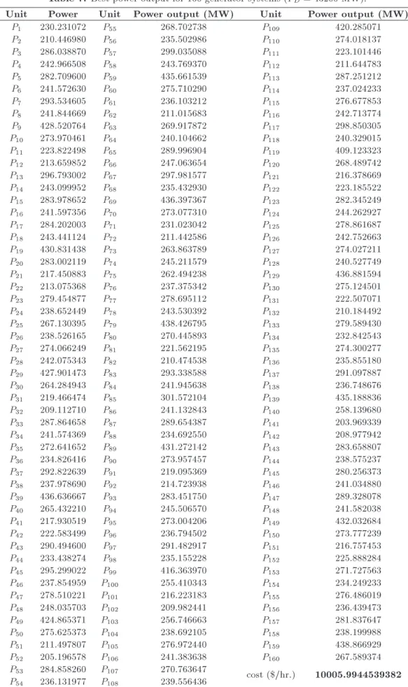
Test system 4: A complex system with 160 ther-mal units is considered here. The input data are available in [31]. The system demand is 43200 MW. Transmission loss has not been included. The best result obtained using the proposed TLBO algorithm is shown in Table 7. Minimum, average and maxi-mum fuel costs obtained by TLBO, ED-DE [31], and dierent GA [31] methods over 50 trials are presented in Table 8. The convergence characteristic of the 160-generator systems obtained by TLBO is shown in Figure 6.

(9)

Table 3. Best power output for 38-generator systems (PD= 6000 MW). Output

(MW) TLBO DE/BBO [27] BBO [27] PSO TVAC [27] NEW PSO [27]

P1 425.891375 426.606060 422.230586 443.659 550.000

P2 426.828618 426.606054 422.117933 342.956 512.263

P3 430.318693 429.663164 435.779411 433.117 485.733

P4 429.480487 429.663181 445.481950 500.00 391.083

P5 429.996241 429.663193 428.475752 410.539 443.846

P6 430.036039 429.663164 428.649254 492.864 358.398

P7 429.142948 429.663185 428.119288 409.483 415.729

P8 428.764849 429.663168 429.900663 446.079 320.816

P9 114.000000 114.000000 115.904947 119.566 115.347

P10 114.000000 114.000000 114.115368 137.274 204.422

P11 119.373112 119.768032 115.418662 138.933 114.000

P12 127.864848 127.072817 127.511404 155.401 249.197

P13 110.000000 110.000000 110.000948 121.719 118.886

P14 90.000000 90.0000000 90.0217671 90.924 102.802

P15 82.000000 82.0000000 82.0000000 97.941 89.0390

P16 120.000000 120.000000 120.038496 128.106 120.000

P17 159.332636 159.598036 160.303835 189.108 156.562

P18 65.000000 65.0000000 65.0001141 65.0000 84.265

P19 65.000000 65.0000000 65.0001370 65.0000 65.041

P20 271.994045 272.000000 271.999591 267.422 151.104

P21 271.999334 272.000000 271.872680 221.383 226.344

P22 259.997110 260.000000 259.732054 130.804 209.298

P23 130.995978 130.648618 125.993076 124.269 85.719

P24 10.000001 10.0000000 10.4134771 11.535 10.000

P25 113.306372 113.305034 109.417723 77.103 60.000

P26 88.045293 88.0669159 89.3772664 55.018 90.489

P27 37.532207 37.5051018 36.4110655 75.000 39.670

P28 20.000000 20.0000000 20.0098880 21.628 20.000

P29 20.000000 20.0000000 20.0089554 29.829 20.995

P30 20.000000 20.0000000 20.0000000 20.326 22.810

P31 20.000000 20.0000000 20.0000000 20.000 20.000

P32 20.000000 20.0000000 20.0033959 21.840 20.416

P33 25.000000 25.0000000 25.0066586 25.620 25.000

P34 18.000000 18.0000000 18.0222107 24.261 21.319

P35 8.000000 8.00000000 8.00004260 9.6670 9.1220

P36 25.000000 25.0000000 25.0060660 25.000 25.184

P37 21.907418 21.7820891 22.0005641 31.642 20.000

P38 21.192396 21.0621792 20.6076309 29.935 25.104

Fuel

cost ($/hr.) 9411938.5572307333 9417235.786391673 9417633.6376443729 9500448.307 9516448.312

Table 4. Comparison between maximum, minimum and average value taken after 50 trials (38-generator systems).

(sec)

solution

deviation

(10)

Table 5. Best power output for 140-generator systems (PD= 49342 MW).

Unit Power output (MW) Unit Power output (MW) Unit Power output (MW)

P1 119.000000 P48 249.994057 P95 837.500000

P2 163.992556 P49 249.946191 P96 682.000000

P3 189.972341 P50 249.929215 P97 720.000000

P4 189.998972 P51 165.209529 P98 718.000000

P5 168.535362 P52 165.011169 P99 720.000000

P6 189.997956 P53 165.016223 P100 964.000000

P7 490.000000 P54 165.451209 P101 958.000000

P8 490.000000 P55 180.017382 P102 947.900000

P9 496.000000 P56 180.022796 P103 934.000000

P10 496.000000 P57 103.221141 P104 935.000000

P11 496.000000 P58 198.019702 P105 876.500000

P12 496.000000 P59 312.000000 P106 880.900000

P13 506.000000 P60 310.335980 P107 873.700000

P14 509.000000 P61 163.059478 P108 877.400000

P15 506.000000 P62 95.011962 P109 871.700000

P16 505.000000 P63 510.936198 P110 864.800000

P17 506.000000 P64 510.798512 P111 882.000000

P18 506.000000 P65 489.960051 P112 94.008366

P19 505.000000 P66 255.973389 P113 94.008341

P20 505.000000 P67 489.682262 P114 94.002109

P21 505.000000 P68 490.000000 P115 244.043393

P22 505.000000 P69 130.012045 P116 244.017301

P23 505.000000 P70 339.411380 P117 244.021535

P24 505.000000 P71 139.530668 P118 95.016467

P25 537.000000 P72 388.321434 P119 95.012018

P26 537.000000 P73 201.593238 P120 116.010750

P27 549.000000 P74 175.736242 P121 175.016446

P28 549.000000 P75 211.418208 P122 2.000193

P29 501.000000 P76 274.267672 P123 4.001186

P30 499.000000 P77 382.327348 P124 15.012599

P31 506.000000 P78 330.234153 P125 9.010491

P32 506.000000 P79 531.000000 P126 12.001651

P33 506.000000 P80 531.000000 P127 10.001491

P34 506.000000 P81 541.971416 P128 112.019297

P35 500.000000 P82 56.003078 P129 4.004812

P36 500.000000 P83 115.032582 P130 5.034679

P37 241.000000 P84 115.003931 P131 5.001229

P38 241.000000 P85 115.027600 P132 50.000415

P39 774.000000 P86 207.012109 P133 5.001042

P40 769.000000 P87 207.012532 P134 42.021338

P41 3.014093 P88 175.000656 P135 42.002799

P42 3.001595 P89 175.148390 P136 41.005287

P43 250.000000 P90 182.053148 P137 17.004924

P44 249.166734 P91 175.129746 P138 7.018298

P45 250.000000 P92 575.400000 P139 7.001898

P46 249.803132 P93 547.500000 P140 26.291702

(11)

(sec)

solution

deviation

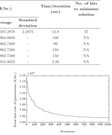
TLBO 1657596.2512 1657586.7157 1657587.2878 2.2875 12.8 47 CTPSO [21] 1658002.7900 1657962.7300 1657964.0600 - 100 NA

CSPSO [21] 1657962.8500 1657962.7300 1657962.7400 - 99 NA

COPSO [21] 1657962.7300 1657962.7300 1657962.7300 - 150 NA CCPSO [21] 1657962.7300 1657962.7300 1657962.7300 - 150 NA MTLA [30] 1657951.9053 1657951.9053 1657951.9053 - 2.28 NA

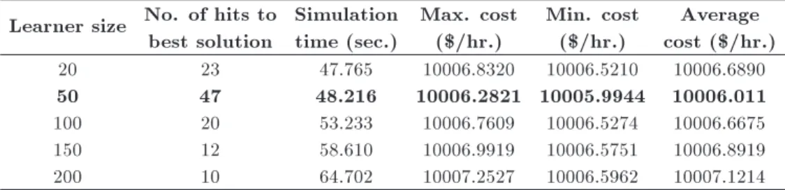
4.2. Eect of learner size for TLBO algorithms

Very large or small values of learner size may not be capable of getting the minimum value of fuel costs. For each learner size of 20, 50, 100, 150 and 200, 50 trials have been run. Out of these, the learner size of 50 achieves the best fuel cost of generations for this system. For other learner sizes, no signicant improve-ment of fuel cost has been observed. Moreover, beyond

Figure 6. Convergence characteristic of 160-generator systems obtained by TLBO.

learner size of 50, simulation time also increases. The best output obtained by the TLBO algorithm for each learner size is presented in Table 9.

4.2.1. Comparative study

1. Solution quality: Tables 1, 3, 5, and 7 present the best fuel cost obtained by TLBO for 4 dierent test systems. The minimum costs obtained for the 4 test system are better, compared to the results obtained by many previously developed techniques, and are also shown in Tables 2, 4, 6 and 8. These tables also represent the comparative studies for maximum, minimum and average values obtained by dierent algorithms. From the results, it is clear that the performance of the TLBO algorithm is better, in terms of quality of solution, compared to many already existing techniques.

2. Computational eciency: In Tables 2, 4, 6 and 8, it is shown that the time taken by TLBO to achieve minimum fuel costs is much less compared to many other techniques. These results prove the signicantly better computational eciency of TLBO.

3. Robustness: The performance of any heuristic algorithm cannot be judged by a single run.

(12)

Nor-Table 7. Best power output for 160-generator systems (PD= 43200 MW).

Unit Power Unit Power output (MW) Unit Power output (MW)

P1 230.231072 P55 268.702738 P109 420.285071

P2 210.446980 P56 235.502986 P110 274.018137

P3 286.038870 P57 299.035088 P111 223.101446

P4 242.966508 P58 243.769370 P112 211.644783

P5 282.709600 P59 435.661539 P113 287.251212

P6 241.572630 P60 275.710290 P114 237.024233

P7 293.534605 P61 236.103212 P115 276.677853

P8 241.844669 P62 211.015683 P116 242.713774

P9 428.520764 P63 269.917872 P117 298.850305

P10 273.970461 P64 240.104662 P118 240.329015

P11 223.822498 P65 289.996904 P119 409.123323

P12 213.659852 P66 247.063654 P120 268.489742

P13 296.793002 P67 297.981577 P121 216.378669

P14 243.099952 P68 235.432930 P122 223.185522

P15 283.978652 P69 436.397367 P123 282.345249

P16 241.597356 P70 273.077310 P124 244.262927

P17 284.202003 P71 231.023042 P125 278.861687

P18 243.441124 P72 211.442586 P126 242.752663

P19 430.831438 P73 263.863789 P127 274.027211

P20 283.002119 P74 245.211579 P128 240.527749

P21 217.450883 P75 262.494238 P129 436.881594

P22 213.075368 P76 237.375342 P130 275.124501

P23 279.454877 P77 278.695112 P131 222.507071

P24 238.652449 P78 243.530392 P132 210.184492

P25 267.130395 P79 438.426795 P133 279.589430

P26 238.526165 P80 270.445893 P134 232.842543

P27 274.066249 P81 221.562195 P135 274.300277

P28 242.075343 P82 210.474538 P136 235.855180

P29 427.901473 P83 293.338588 P137 291.097887

P30 264.284943 P84 241.945638 P138 236.748676

P31 219.466474 P85 301.572104 P139 435.188836

P32 209.112710 P86 241.132843 P140 258.139680

P33 287.864658 P87 289.654387 P141 203.969339

P34 241.574369 P88 234.692550 P142 208.977942

P35 272.641652 P89 431.272142 P143 283.658807

P36 234.826416 P90 273.957457 P144 238.575237

P37 292.822639 P91 219.095369 P145 280.256373

P38 237.978690 P92 214.723938 P146 241.034880

P39 436.636667 P93 283.451750 P147 289.328078

P40 265.432210 P94 245.506570 P148 241.582038

P41 217.930519 P95 273.004206 P149 432.032684

P42 222.583499 P96 236.794502 P150 273.777239

P43 290.494600 P97 291.482917 P151 216.757453

P44 233.438274 P98 235.155228 P152 225.888284

P45 295.299022 P99 416.363970 P153 271.727563

P46 237.854959 P100 255.410343 P154 234.249233

P47 278.510221 P101 216.223183 P155 276.486019

P48 248.035703 P102 209.982441 P156 236.439473

P49 424.865371 P103 256.746663 P157 281.837647

P50 275.625373 P104 238.692105 P158 238.199988

P51 211.497807 P105 276.972440 P159 438.866929

P52 205.196578 P106 241.383638 P160 267.589374

P53 284.858260 P107 270.763647 _{cost ($/hr.)} _{10005.9944539382} P54 236.131977 P108 239.556436

(13)

(Sec)

solution

deviation

TLBO 10006.28210000 10005.9944539382 10006.01170000 0.0690 48.216 47

ED-DE [31] NA 10012.68 NA - NA NA

CGA-MU [31] NA 10143.73 NA - NA NA

IGA-MU [31] NA 10042.47 NA - NA NA

Table 9. Eect of learner size on 160-generator systems. Learner size No. of hits to

best solution

Simulation time (sec.)

Max. cost ($/hr.)

Min. cost ($/hr.)

Average cost ($/hr.)

20 23 47.765 10006.8320 10006.5210 10006.6890

50 47 48.216 10006.2821 10005.9944 10006.011

100 20 53.233 10006.7609 10006.5274 10006.6675

150 12 58.610 10006.9919 10006.5751 10006.8919

200 10 64.702 10007.2527 10006.5962 10007.1214

mally, their performance is judged after running the programs for a certain number of trials. A great number of trials should be made to obtain a useful conclusion about the performance of the algorithm. An algorithm is said to be robust if it gives consis-tent results during these trial runs. Tables 2, 4, 6 and 8 show that out of 50 trials for four dierent test systems, TLBO reaches minimum costs 50, 50, 47 and 47 times, respectively. The eciency of the TLBO algorithm to reach minimum solution is 100% and 94%, respectively. This performance is far superior to many other algorithms presented in dierent literature. Therefore, the above results establish the enhanced ability of TLBO to achieve superior quality solutions, in a computationally ecient and robust way.

5. Conclusion

In the present paper, a newly developed TLBO algo-rithm has been successfully implemented in the eld of power systems to solve dierent convex and non-convex ELD problems. The simulation results show that the performance of TLBO is better compared to that of several previously developed optimization techniques. The TLBO has obtained superior quality solutions with high convergence speed in a very robust way. The results also show the advantage of TLBO, compared to many previously developed optimization techniques, in term of computational time, as the proposed algorithm is parameter free. Therefore, TLBO can be considered to be a strong tool for solving complex ELD problems. Moreover, the successful implementation and superior performance of TLBO to solve ELD problems has

created a new path in the eld of power systems, which may encourage the researcher to apply this newly developed algorithm to solve dierent, greatly complex power system optimization problems, like optimal power ow, hydro thermal scheduling, loss minimization, optimal placement of distributed genera-tors, and FACTS devices etc. Therefore, it may nally be concluded that the proposed TLBO algorithm is able to solve any complex constrained optimization problem with a faster convergence rate, irrespective of the nature of the objective function.

References

1. El-Keib, A.A., Ma, H. and Hart, J.L. \Environmen-tally constrained economic dispatch using the La-grangian relaxation method", IEEE Trans PWRS, 9(4), pp. 1723-1729 (1994).

2. Fanshel, S. and Lynes, E.S. \Economic power gener-ation using linear programming", IEEE Transactions on Power Apparatus and Systems PAS, 83(4), pp. 347-356 (1964).

3. Wood, J. and Wollenberg, B.F., Power Generation, Operation, and Control, John Wiley and Sons, 2nd Ed. (1984).

4. Walters, D.C. and Sheble, G.B. \Genetic algorithm so-lution of economic dispatch with valve point loadings", IEEE Trans PWRS, 8(3), pp. 1325-1331 (1993).

5. Bakirtzis, A., Petridis, V. and Kazarlis, S. \Genetic algorithm solution to the economic dispatch problem, generation transmission and distribution", IEE pro-ceeding, 141(4), pp. 377-382 (1994).

6. Gaing, Z.L. \Particle swarm optimization to solving the economic dispatch considering the generator

(14)

con-straints", IEEE Trans PWRS, 18(3), pp. 1187-1195 (2003).

7. Hou, Y.H., Wu, Y.W., Lu, L.J. and Xiong, X.Y. \Generalized ant colony optimization for economic dis-patch of power systems", Proceedings of International Conference on Power System Technology Power-Con, 1, pp. 225-229 (2002).

8. Jayabharathi, T., Jayaprakash, K., Jeyakumar, N. and Raghunathan, T. \Evolutionary programming techniques for dierent kinds of economic dispatch problems", Elect. Power Syst. Res., 73(2), pp. 169-176 (2005).

9. Panigrahi, C.K., Chattopadhyay, P.K., Chakrabarti, R.N. and Basu, M. \Simulated annealing technique for dynamic economic dispatch", Electric Power Compo-nents and Systems, 34(5), pp. 577-586 (2006).

10. Nomana, N. and Iba, H. \Dierential evolution for economic load dispatch problems", Elect. Power Syst. Res., 78(3), pp. 1322-1331 (2008).

11. Panigrahi, B.K., Yadav, S.R., Agrawal, S. and Tiwari, M.K. \A clonal algorithm to solve economic load dispatch", Elect. Power Syst. Res., 77(10), pp. 1381-1389 (2007).

12. Panigrahi, B.K. and Pandi, V.R. \Bacterial foraging optimization: Nelder-Mead hybrid algorithm for eco-nomic load dispatch", IET Generation, Transmission, Distribution, 2(4), pp. 556-565 (2008).

13. Bhattacharya, A. and Chattopadhyay, P.K. \Biogeography-based optimization for dierent economic load dispatch problems", IEEE Trans PWRS, 25(2), pp. 1064-1077 (2010).

14. Chiang, C.L. \Improved genetic algorithm for power economic dispatch of units with valve-point eects and multiple fuels", IEEE Trans PWRS, 20(4), pp. 1690-1699 (2005).

15. Alsumait, J.S., Sykulski, J.K. and Al-Othman, A.K. \A hybrid GA-PS-SQP method to solve power system valve-point economic dispatch problems", Appl. En-ergy, 87(5), pp. 1773-1781 (2010).

16. Sinha, N., Chakrabarti, R. and Chattopadhyay, P.K. \Evolutionary programming techniques for economic load dispatch", IEEE Trans. Evol. Comput., 7(1), pp. 83-94 (2003).

17. Selvakumar, A.I. and Thanushkodi, K. \A new particle swarm optimization solution to nonconvex economic dispatch problems", IEEE Trans PWRS, 22(1), pp. 42-51 (2007).

18. Panigrahi, B.K., Pandi, V.R. and Das, S. \Adaptive particle swarm optimization approach for static and dynamic economic load dispatch", Energy Conver. & Managt., 49(6), pp. 1407-15 (2008).

19. Chaturvedi, K.T., Pandit, M. and Srivastava, L. \Self-organizing hierarchical particle swarm optimization for nonconvex economic dispatch", IEEE Trans PWRS, 23(3), pp. 1079-1087 (2008).

20. Vlachogiannis, J.G. and Lee, K.Y. \Economic load dis-patch - A comparative study on heuristic optimization techniques with an improved coordinated aggregation-based PSO", IEEE Trans PWRS, 24(2), pp. 991-1001 (2009).

21. Park, J.B., Jeong, Y.W., Shin, J.R. and Lee, K.Y. \An improved particle swarm optimization for nonconvex economic dispatch problems", IEEE Trans PWRS, 25(1), pp. 156-166 (2010).

22. Lu, H., Sriyanyong, P., Song, Y.H. and Dillon, T. \Ex-perimental study of a new hybrid PSO with mutation for economic dispatch with non-smooth cost function", Int. J. Elect. Power Energy Syst., 32(9), pp. 921-935 (2010).

23. Coelho, L.D.S. and Mariani, V.C. \Combining of chaotic dierential evolution and quadratic program-ming for economic dispatch optimization with valve-point eect", IEEE Trans PWRS, 21(2), pp. 989-996 (2006).

24. Chiou, J.P. \Variable scaling hybrid dierential evo-lution for large-scale economic dispatch problems", Elect. Power Syst. Res., 77(3-4), pp. 212-218 (2007).

25. Duvvuru, N. and Swarup, K.S. \A hybrid interior point assisted dierential evolution algorithm for eco-nomic dispatch", IEEE Trans PWRS, 26(2), pp. 541-549 (2011).

26. Panigrahi, B.K. and Pandi, V.R. \Bacterial foraging optimisation: Nelder-Mead hybrid algorithm for eco-nomic load dispatch", IET Gener. Transm. Distrib., 2(4), pp. 556-565 (2008).

27. Bhattacharya, A. and Chattopadhyay, P.K. \Hybrid dierential evolution with biogeography-based opti-mization for solution of economic load dispatch", IEEE Trans PWRS, 25(4), pp. 1955-1964 (2010).

28. Rao, R.V., Savsani, V.J. and Vakharia, D.P. \Teaching-learning-based optimization: A novel method for constrained mechanical design optimiza-tion problems", Computer-Aided Design, 43(3), pp. 303-315 (2011).

29. Yang, H.T., Yang, P.C. and Huang, C.L. \A parallel genetic algorithm approach to solving the unit com-mitment problem: Implementation on the transputer networks", IEEE Trans. Power Syst., 12(2), pp. 661-668 (1997).

30. Niknam, T., Azizipanah-Abarghooee, R. and Aghaei, J. \A new modied teaching-learning algorithm for re-serve constrained dynamic economic dispatch", IEEE Trans. Power Syst., 28(2), pp. 749-763 (2013).

31. Wang, Y., Li, B. and Weise, T. \Estimation of distri-bution and dierential evolution cooperation for large scale economic load dispatch optimization of power systems", Information Sciences, 180(12), pp. 2405-2420 (2010).

Biographies

Kuntal Bhattacharjee received a BE degree from BIET, Suri Private College (Burdwan University), and

(15)

an M.Tec degree from NIT, Durgapur, India, in 2003 and 2005, respectively, all in Electrical Engineering. He is currently in the Electrical Engineering Department at Dr. B.C. Roy Engineering, Durgapur, India. His research interests include power system optimization, ELD, EELD, and hydrothermal applications.

Aniruddha Bhattacharya received BSc. Engg. degree in Electrical Engineering from the Regional Institute of Technology, Jamshedpur, India, in 2000, an ME degree in Electrical Power Systems, and a PhD degree from Jadavpur University, Kolkata, India, in 2008 and 2011 respectively.

He is currently working as Assistant Professor in the Electrical Engineering Department at the National Institute of Technology, Agartala, Tripura, India. His employment experience includes Siemens Metering Limited, India; Jindal Steel & Power Limited, Raigarh,

India; Bankura Unnyani Institute of Engineering, Bankura, India; and Dr. B.C. Roy Engineering College, Durgapur, India. His areas of interest include power system load ow, optimal power ow, economic load dispatch, hydro thermal scheduling, power system reliability and soft computing applications to dierent power system problems.

Sunita Halder (nee Dey) received a BE degree from Jalpaiguri Government College in 1998, and ME and PhD degrees from BESU, Kolkata, India, in 2001 and 2006, respectively, all in Electrical Engineering. She is currently with the Electrical Engineering Department at Jadavpur University, Kolkata India. She has pub-lished and presented several research papers in inter-national and inter-national journals and at conferences. Her research interests include power system operation and control, OPF, voltage stability, FACTS applications.