c
Sharif University of Technology, October 2010
Solution of Convection-Dominated Problems
on Irregular Meshes by Collocated Discrete
Least Squares Mesh-Less (CDLSM) Method
M.H. Afshar
1and G. Shobeyri
1;Abstract. In this paper, a study is performed on the eect of irregularity of domain discretization on the performance of the CDLSM method for the solution of convection-dominated problems. The method is based on minimizing a least squares functional of the residuals of the governing dierential equations and its boundary conditions over a set of collocation points. Four convection-dominated benchmark examples are solved using CDLSM method on three dierent sets of nodal distribution with dierent levels of irregularity and the results are presented. These experiments show that CDLSM method is capable of producing stable and accurate results for hyperbolic problems with shocked or high gradient solutions even on highly irregular mesh of nodes. Mesh-less methods as alternative numerical approaches to eliminate the well-known drawbacks of mesh-based methods have attracted much attention in the past decade due to their exibility and their potentiality in negating the need for the human-labor intensive process of constructing geometric meshes in a domain. Exploiting this ability, however, requires that the method could solve the problem under consideration on unstructured distribution of nodes. This is particularly important when a renement strategy is to be used to improve the performances of these methods. Keywords: CDLSM; Meshless; Irregular mesh; Convection-dominated problems; Renement strategy.
INTRODUCTION
In the past decades, a group of so-called mesh-free or meshless methods have become one of the hottest areas of research in computational mechanics. As their name implies, one common characteristic of all these methods is that they do not require the traditional mesh to construct the numerical formulation. Mesh-free meth-ods possess a number of interesting properties. For example, they require node generation instead of mesh generation. In other words, there is no pre-specied connectivity or relationship among the nodes, thus the computational costs associated with mesh generation are highly reduced. Another attractive property of mesh-free methods is the computational ease of adding and subtracting nodes from the pre-existing nodes. The computational advantages of a mesh-free method suggest that they have potentials in solving a broad class of scientic and engineering problems.
1. School of Civil Engineering, Iran University of Science and Technology, Tehran, P.O. Box 16765-163, Iran.
*. Corresponding author. E-mail: [email protected]
Received 28 September 2009; received in revised form 12 June 2010; accepted 26 July 2010
Various meshless methods have been developed and used to solve dierent problems including those encountered in the uid mechanics discipline. Smooth Particle Hydrodynamics (SPH) introduced by Gingold and Monaghan [1], and used by Ataie and Shobeyri [2] and Ataie et al. [3], Reproducing Kernel Particle Method (RKPM) by Liu et al. [4], Element-Free Galerkin method (EFG) by Belytschko et al. [5], Mesh-less Local Petrov-Galerkin (MLPG) method by Atluri and Zhu [6], partition of unity by Melenk and Babuska [7], Hp-clouds by Duarte and Oden [8] and Finite Point (FP) method by Onate et al. [9] are all meshless methods from the point of view of the node interpolation, and have already been widely applied to various areas. The advantages of these meshless meth-ods are apparent, however, serious limitations exist. For instance, the diculties of imposition of essential boundary and treatment of material discontinuities, uncertain choice of the weight functions, diculties in the integration of stiness matrix, and complexity in algorithms for computing the interpolation functions are all major technical problems in these methods.
The meshless methods have been proposed to avoid the numerical diculties of mesh entanglement
in the Finite Element Method (FEM) which have been widely used in dierent engineering elds [10-12]. Meshless methods, however, have to pay for the high cost in the computational time, the enforcement of essential boundary condition and the treatment of ma-terial discontinuities. Special technologies, such as the Penalty method by Zhu and Atluri [13], transformation of approximate nodal values to actual nodal values by Cai and Zhu [14], nodal integration method by Beissel and Belytschko [15], and ecient computation of shape functions by Beitkopf et al. [16] have been proposed to overcome these problems.
Recently a family of collocation-based meshless methods are emerging in the literature. Collocation methods enjoy simplicity and eciency when used as meshless methods but they suer from stability problems. Some researchers have, therefore, attempted a hybridization of the collocation method with other discretization schemes as a remedy to the shortcomings of the collocation methods. Afshar and Arzani [17] developed Discrete Least Squares Mesh-less (DLSM) method for the solution of Poisson equation. In this method a fully least squares approach was used in both function approximation and the discretization of the governing dierential equations. The meshless shape functions were derived using the Moving Least Squares (MLS) method of function approximation. The discretized equations were obtained via a discrete least squares method in which the sum of the squared residuals were minimized with respect to the unknown nodal parameters. While most of the existing meshless methods need background cells for numerical inte-gration, DLSM did not require numerical integration procedure. This method had the additional advantages of producing symmetric, positive and denite matrices even for non-self adjoint operators as encountered in uid ow problems.
Zhang et al. used the Least squares Collocation Meshless (LSCM) Method [18] to solve elliptic prob-lems. In this method, a set of over determined system of equations, in which the number of the equations was greater than the number of unknowns, was con-structed and solved by the least squares method. The solution of some steady and unsteady heat conduction problems were investigated by Liu et al. [19] using a Meshless Weighted Least Squares (MWLS) method. A sensitivity analysis on the MWLS parameters to solve the problems of a cantilever beam and an innite plate with a central circular hole was performed by Pan et. al [20]. Armentano and Duran [21] carried out an error estimates for moving least square approximations used for the solution of 1-D convection-diusion problems. Wang et al. [22] tested a point weighted least squares meshless method for the solution of 1-D and 2-D Poisson equations.
Firoozjaee and Afshar [23] proposed Collocated
Discrete Least Squares Mesh-less (CDLSM) method to solve elliptic partial dierential equations, and studied the eect of the collocation points on the convergence and accuracy of the method. CDLSM was later extended by Naisipour et al. [24] to solve elasticity problems on irregular distribution of nodal points. Afshar and Lashckarbolok [25] were rst to use the CDLSM method for the solution of hyperbolic problems. They also suggested a posteriori error estimate and adaptive renement strategy in conjunc-tion with the CDLSM method for 1-D hyperbolic problems. More recently, Afshar et al. [26] examined the eect of the number of collocation points on the accuracy of CDLSM method for both transient and steady state one dimensional hyperbolic problems with uniform nodal spacing. CDLSM has also been used successfully to simulate free surface ows by Shobeyri and Afshar [27].
CDLSM has shown to have some similarity with MWLS as suggested by Liu et al. [19] and Pan et al. [20] who use least squares method for the discretization of the governing dierential equations. A simple but very decisive dierence, however, exists between these methods which is the use of the collocation points in the CDLSM method. In CDLSM, the least squares functional is formed at the collocation points while it is calculated at nodal points in MWLS. At least three advantages of the collocation points were shown in [26] which are as follows. First, the collocation points can stabilize the method, especially in problems with shocked solution. Second, the collocation points can improve the accuracy of the method even in problems with smooth solutions. Third, faster convergence can be achieved in steady-state problems using collocation points. It has recently, however, come to the attention of the authors, by one of the respected reviewers of the paper, that in an alternative formulation of the MWLS method proposed by Zhang et al. [28], a set of auxiliary points in addition to the nodal points were also used to eliminate the residuals of the governing equations.
In this paper, the CDLSM method is extended for the solution of one and two dimensional convection dominated problems and its performance for the so-lution of steady and transient problems on irregular distribution of nodes are investigated. Four test problems from the literature, namely nonlinear 1-D Burgers equation in transient form, 1-D dam break problem, 2-D pure convection problem and nally 2-D transient Burgers equation are solved using proposed CDLSM method on three set of node congurations with dierent level of irregularity and the results are presented and compared to the analytical results wherever available. These experiments show that the proposed CDLSM method is capable of producing stable and accurate results for the dicult problems considered.
MOVING LEAST SQUARES (MLS) METHOD
Several techniques have been developed to construct meshless shape functions. The MLS approximation by Lancaster and Salkauskas [29], the Radial Point Interpolation Method (RPIM) by Liu and Gu [30] and the Kriging interpolation by Gu [31] are only some examples of existing methods. Amongst these methods, the MLS method has gained more popularity in the meshless community. In MLS, the function to be approximated is represented by:
uh(x) =Xm i=1
pi(x)ai(x) pT(x)a(x): (1)
Here pT(x) is a set of linearly independent polynomial
basis and a(x) represents the unknown coecients to be determined by the tting algorithm. In Moving Least Square (MLS) approximation, at each point x, a(x) is chosen to minimize the sum of weighted squared residuals dened by:
J = 12
n
X
I=1
w(jx xIj)[pT(xI)a(x) uI]2; (2)
where uI is nodal value of the function to be
approx-imated, n is the number of nodes and w(jx xIj) is
the weight function dened to have compact support. Many weight functions are established and used by dierent researchers. In this paper an exponential weight function is used as follows:
w(r) = 8 > < > : 2
3 4r2+ 4r3 for r 12 4
3 4r + 4r2 43r3 for 12 < r 1
0 for r > 1
(3) in which r = s=smax, s = kx xIk and smax is the
radius of the support.
The coecients a(x) are found by minimizing J with respect to these coecients. Carrying out the dierentiation and setting it to zero leads to the following relation for the unknown parameters a(x):
a(x) = A 1(x)B(x)u; (4)
where:
A = PTW(x)P; (5)
B = PTW(x); (6)
uT = (u
1; u2; ; un); (7)
P = 2 6 6 6 4
p1(x1) p2(x1) pm(x1)
p1(x2) p2(x2) pm(x2)
... ... ... ...
p1(xn) p2(xn) pm(xn)
3 7 7 7
5; (8)
and: W(x) = 2 6 6 6 4
w(jx x1j) 0 0
0 w(jx x2j) 0
... ... ... ...
0 0 w(jx xnj)
3 7 7 7 5: (9) The approximation of the unknown function can now be written in the familiar form of:
uh(x) =Xn I=1
NI(x)uI; (10)
where NI(x) denote the shape function of node I
dened as:
N = pT(x)A 1(x)B(x): (11)
MLS shape functions generally do not satisfy the Kronecker delta condition. Hence the parameters uI
cannot be treated like nodal values of the unknown function (uh(x
i) 6= uI).
Generally, it is necessary to obtain the shape function derivatives. The spatial derivatives of the shape functions are obtained as:
dN(x)
dx =
dP
dxA 1B + P d(A 1)
dx B + PA 1
dB dx: (12) COLLOCATED DISCRETE LEAST
SQUARES MESHLESS (CDLSM) METHOD Consider the general form of dierential equations governing the transient convection-diusion problems written in matrix form as:
@u
@t + Ai(u) @u @xi k
@2u
@x2
i = Q(u);
i = 1; 2; on : (13)
Subject to appropriate Dirichlet and Neuman bound-ary conditions:
u = u on u;
B(u) = g on t:
(14) Here, u denotes the problem unknown vector, Aiis the
Jacobian matrix in the ith dimension which is generally a function of the unknown vector u, Q is the source term vector, k is the diusion coecient assumed to be independent from the spatial dimensions and B is a dierential operator dened on Neuman boundaries.
A semi-discretization is rst carried out using the method in time as follows:
un+1 un
+t
An+1 i (u)@u
n+1
@xi k
@2un+1
@x2 i Q n+1 +t(1 ) An i(u)@u
n
@xi k
@2un
@x2 i Q
n=0;
(15) with 1
2 1 for the stability of the temporal
dis-cretization scheme. Assuming Q = Su, the linearized residuals in the problem domain and its boundaries can now be dened as:
Rn+1
= un+1 un
+ t
An i(u)@u
n+1
@xi k
@2un+1
@x2 i S
nun+1
+t(1 )
An i(u)@u
n
@xi k
@2un
@x2 i S
nun;
(16) Rn+1
t = B(uk) g(xk); (17)
Rn+1
u = u
n+1 u: (18)
The philosophy of least squares is to nd an approx-imate solution that minimizes the least squares func-tional to be dened later. Assume that the problem domain and boundaries are discretized by some nodal points, and their number is n. Beside the nodal points, the collocation points are used in the problem domain and on its boundaries to construct the least squares functional. The total number of collocation points is M comprised of Md internal collocation points, Mu
collocation points on the Dirichlet boundary and Mt
collocation points on Neuman boundary, i.e.:
M = Md+ Mu+ Mt: (19)
The approximate value of the function u at a colloca-tion point xkcan be obtained through interpolation:
u(xk) = nk
X
i=1
Ni(xk):ui; (20)
where nk is the number of nodal points having xk
in their support domain. Substituting Equation 20 into Equations 16, 17 and 18 leads to the dierential equation residual Rd, the Neuman boundary condition
residual Rtand the Dirichlet boundary condition
resid-ual Ru dened as:
R(d)k = L(uk) f(xk) = nk
X
j=1
L(Nj(xk))uj f(xk);
(k = 1 M); (21)
with
L() = () + t
An i(u)@()@x
i k
@2()
@x2 i S
n();
(22) f = un t(1 )An
i @u n
@xi k
@2un
@x2 i Q
n; (23)
R(t)k =B(uk) g(xk)= nk
X
j=1
B(Nj(xk))uj g(xk);
(k = 1 Mt); (24)
R(u)k = uk u = nk
X
j=1
(Nj(xk))uj u;
(k = 1 Mu): (25)
Now the least squares functional of all residuals at all collocation points can be constructed as:
J =12 XMd
k=1
[R(d)k ]2+XMt k=1
[R(t)k ]2+:XMu k=1
[R(u)k ]2
! :
(26) The factors and in the above equation are meant to represent the relative weight of the boundary residuals with respect to the domain residual.
Minimization of Equation 26 with respect to the nodal parameters ui leads to:
@J @ui =
M
X
k=1
@R(d)k @ui [R
(d) k ] +
Mt
X
k=1
@Rk(t) @ui [R
(t) k ]
+ XMu
k=1
@R(u)k @ui [R
(u)
k ] = 0: (27)
Substituting Equations 21, 24 and 25 into Equation 27 yields the nal system of equations:
KU = F: (28)
The typical components of the matrix K and right hand side vector F are dened as:
Klm = Md
X
i=1
[L(Nl)]Ti[L(Nm)]i
+
Mt
X
i=1
[B(Nl)]Ti [B(Nm)]i
+ XMu
i=1
[(Nl)]Ti[(Nm)]i;
Fl= Md
X
i=1
[L(Nl)]Ti fi+ Mt
X
i=1
[B(Nl)]Tigi
+ XMu
i=1
[(Nl)]Ti(u);
l = 1; ; n: (30)
The system of equations can now be formed and solved at each time step and the required solution produced in a time marching manner until a steady state solution is reached if a steady state solution is desired. It should be noted here that the proposed method is stable for any time and space step sizes due to the implicit nature of the method. The stiness matrix K in Equation 29 can be seen to be symmetric and positive-denite. Therefore, the nal system of equations can be solved using ecient iterative procedure such as conjugate gradient methods.
NUMERICAL EXAMPLES
In this section, a set of transient and steady state hyperbolic problems are solved on a series of nodal distributions with dierent level of irregularity and the results are compared to assess the eect of mesh ir-regularity on the performance of the proposed CDLSM method. In 1-D problems, the standard deviation of the nodal spacing is considered as a measure of mesh irregularity while for 2-D problems, the average value of the absolute dierence between the radius of support domain on irregular mesh with those on regular mesh is considered as the mesh irregularity.
The mesh irregularity index can be dened math-ematically as:
For one-dimensional problems: Iindx= M 1
n 1 Mn
X
i=1
(xreg
i xirregi )2
!1 2
: For two-dimensional problems:
Iindx= M1 n
Mn
X
i=1
(abs(sreg
maxji sirregmaxji));
where Mn is the number of nodal points in the
com-putational domain, xregi , sreg
maxji, xirregi and sirregmaxji are
the positions of nodal points and the radius of support domain for regular and irregular nodal distributions, respectively.
The accuracy of MLS interpolation greatly dead-ens on how to dene support domain for the point of interest. Therefore, an ecient method to choose
support domain is required for accurate and ecient approximation. For one-dimensional problems, the size of the support domain (smax) is dened so that
at least two nodes be in the support domain. For two-dimensional problems, the radius of the support domain is dened by:
smax= sdc;
where s is a user-dened coecient and dc is a
measure of the average nodal spacing. For irregular nodal point distributions dc is chosen as the average
distance of the ve nearest nodal points to the point under consideration. Generally, s= 2:0 3:0 leads to
accurate results for many problems [32]. Here, s= 2:0
and 2:7 are used for pure convection and the Burgers problems, respectively.
It also should be noted that polynomial basis of order zero (P = [1]) and order two (p = [1; x; y; xy; x2; y2]) are used for 1-D and 2-D problems, respectively,
to construct MLS shape functions. Transient 1-D Burgers Equation
This is a problem governed by the inviscid Burgers equation dened by following parameters of Equa-tion 13:
A = u; k = 0; Q = 0:
The problem is solved on the domain 0 x 1 with the following initial and boundary conditions:
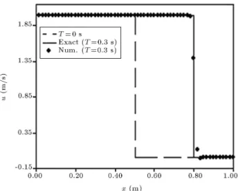
u(0) = 2; 0 x 0:5; u(0) = 0; 0:5 < x 1; u(t) = 2; x = 0:0; u(t) = 0; x = 1:
The exact solution to this problem is represented by a discontinuity moving with velocity of 1 m/s. Burgers equation is a simple non-linear model representing physical problems described by the convection-diusion and convection-reaction process. Many physical prob-lems such as sound and shock waves in viscous medium and magnetohydrodynamic waves can be described by Burgers equation.
This problem is solved on a mesh of 61 nodal points with 121 distributed collocation points, 61 of them coinciding with the nodal points and each of the remaining collocation points is located between two nodal points. The problem is solved on three meshes of 0.0, 0.0078, and 0.0098 irregularity using a time step size of 0.003. The mesh of nodes and the corresponding results are shown in Figures 1 to 3 and
Figure 1. Solution of steady Burgers problem on a mesh of 0.0 irregularity (uniform mesh).
Figure 2. Solution of steady Burgers problem on a mesh of 0.0078 irregularity.
Figure 3. Solution of steady Burgers problem on a mesh of 0.0098 irregularity.
compared with the analytical solution at time of 0.3 s. The results clearly show the ability of the proposed CDLSM method to correctly capture the shock even for highly irregular mesh of Figure 3.
Breaking of a Dam
The non-linear shallow-water equations in one dimen-sion governing the breaking of a dam problem can be dened by the following parameters of Equation 13:
u =
H + (H + )u
; k = 0;
A =
0 1
u2+ g(H + ) 2u
; Q =
0 g(H + )dH=dx
;
where H is the depth, is the surface elevation, u is the velocity, g is the acceleration due to gravity and
dH
dx = 0 is the bed slope. The breaking of a dam
is a signicant practical problem in civil engineering. It is necessarily required to predict the uid ow induced by breaking of dam for designing a dam and its surrounding environment. Dam break ow is an ideal test problem to examine the accuracy of numerical approaches, and it can be simulated by removal of a barrier holding a body of water at rest in numerical simulations.
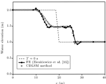
The problem of a propagating jump disconti-nuity due to the breaking of a dam was computed by Lonher et al. [33] using a Taylor-Galerkin nite element method, Carrey and Jiang [34], Zienkiewicz and Taylor [35] and Afshar and Morgan [36] using least square nite element schemes. In the present study, the initial condition of u = 0, = 2 for 0 x 20 and u = 0, = 0 for 20 < x 40 was used. The depth H and g are assumed constant and equal to unity. The problem is solved here on a mesh of 81 nodal points with 321 distributed collocation points, 81 of them coinciding with the nodal points. The problem is solved on three meshes of 0.0, 0.22, and 0.41 irregularity using a time step size of 0.1. The mesh of nodes and the corresponding results are shown in Figures 4 to 6 and compared with the results of Zienkiewicz and Taylor [35]. The results again show that proposed CDLSM method can handle propagating shocked solution on highly irregular meshes.
Two-Dimensional Pure Convection Problem Pure convection problems in 2-D can be described by the following parameters of Equation 13:
Figure 4. Solution of dam break equation problem at T = 5 s on a mesh 0.0 irregularity (uniform mesh).
Figure 5. Solution of dam break equation problem at T = 5 s on a mesh 0.22 irregularity.
Figure 6. Solution of dam break equation problem at T = 5 s on a mesh 0.41 irregularity.
where A1 and A2 are constant coecient representing
the components of the velocity eld along x and y axes, respectively. The boundary conditions of the problem are dened as:
(
u = 0 x = 0; 0 y 1 u = 1 y = 0; 0 x 1
Viscosity eects are neglected in pure convection problems and, therefore, the mathematical solution of these types of problems can be sharp fronts and discontinuities. Viscosity plays a signicant role to smooth the sharp discontinuities in the real physical phenomena.
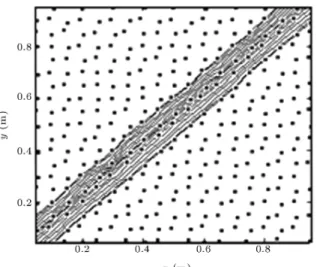
The problem is rst solved on a regular mesh of 441 nodal points (x = y = 0:05) using 841 uniformly distributed collocation points 441 of which coinciding with the nodal points. Figure 7 shows the distribution of nodal points along with the contour lines of solution obtained. This solution was obtained using a time step size of 0.015 and = 0:5.
The problem is also solved on two meshes with irregularity indexes of 0.011 and 0.0195 using the same computational parameters as used on the uniform mesh. Again 841 collocation points are used as in the case of uniform mesh so that the computational eort is the same as that of uniform mesh. 441 of the collocation points coincided with the nodal points and the remaining 400 collocation points were distributed uniformly on the computational domain. Figures 8 and 9 show the nodal distribution and the solution contours on two irregular meshes used. The solutions along y = 0:5 obtained using dierent meshes are compared in Figure 10 showing that the accuracy of the results produced by proposed CDLSM method is not aected much by the irregularity of the meshes used.
Figure 7. Solution of pure convection problem on uniform mesh.
Figure 8. Solution of pure convection problem on a mesh 0.011 irregularity.
Figure 9. Solution of pure convection problem on a mesh 0.0195 irregularity.
Figure 10. Comparison of solution of pure convection problem on dierent meshes.
2-D Viscous Burgers Equation
2-D viscous Burgers equation can be represented by the following parameters of Equation 13.
A1(u) = A2(u) = u; Q(u) = 0:
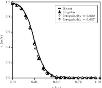
The exact solution of the problem is dened as fol-lows [37]:
u(x; y; t) = 1 + e(x+y t 0:25)=(2k)1 : (31) From which the initial and boundary conditions can be dened.
The computational parameters of = 0:5, t = 0:01 and k = 0:03 were used on three meshes of irreg-ularity indexes 0.0, 0.02 and 0.057, respectively, to get the solution at time t = 0:5 seconds. Figures 11 to 13 shows the contours of the solutions obtained on three
Figure 11. Solution of 2-D Burgers problem at t = 0:5 s on a regular mesh.
Figure 12. Solution of 2-D Burgers problem at t = 0:5 s on a mesh of 0.02 irregularity.
Figure 13. Solution of 2-D Burgers problem at t = 0:5 s on a mesh of 0.057 irregularity.
Figure 14. Comparison of exact and numerical solutions obtained on dierent meshes at t = 0:5 s.
meshes of 441 nodal points using 841 collocation points. Once again 441 of the collocation points coincided with the nodal points while the 400 remaining points was considered to be uniformly distributed on the domain. A comparison of the solutions obtained along y = 0:5 with that of exact solution is shown in Figure 14, indicating the ability of the method to produce nearly exact solution irrespective of the irregularity of the meshes used.
CONCLUDING REMARKS
A fully least squares approach named Collocated Dis-crete Least Squares Mesh-less (CDLSM) method was used in this paper for the solution of convection-dominated problems on irregular meshes. In this method a fully least squares approach is used in both function approximation and the discretization of the
governing dierential equations. The meshless shape functions were derived using the Moving Least Squares (MLS) method of function approximation. The prob-lem domain was discretized by nodal points which are used to construct the trial function. The least square functional is constructed using collocation points that are basically independent of the nodal points. A study is performed on the eect of irregularity of domain discretization on the performance of the proposed Collocated Discreet Least Square Mesh-less (CDLSM) method. Four benchmark examples of hyperbolic nature, namely steady nonlinear 1-D Burgers equation, 1-D dam break problem, 2-D pure convection problem and 2-D viscous Burgers equation were solved on three meshes of dierent irregularity, and the results were presented and compared with the exact solutions where available. The results clearly indicated that the proposed CDLSM method is able to produce highly accurate results for hyperbolic problems even on highly irregular meshes of nodes.
REFERENCES
1. Gingold, R.A. and Moraghan, J.J. \Smooth particle hydrodynamics: theory and application to non spheri-cal stars", Man. Not. Roy. Astron. Soc., 181, pp. 375-389 (1977).
2. Ataie-Ashtiani, B. and Shobeyri, G. \Numerical sim-ulation of landslide impulsive waves by incompress-ible smoothed particle hydrodynamics", International Journal For Numerical Methods in Fluids, 56(2), pp. 209-232 (2008).
3. Ataie-Ashtiani, B., Shobeyri, G. and Farhadi, L. \Modied incompressible SPH method for simulating free surface problems", Fluid Dynamic Research, 40, pp. 637-661 (2008).
4. Liu, W.K., Jun, S. and Zhang, Y. \Reproducing kernel particle methods", Int. J. Numer. Meth. Eng., 20, pp. 1081-1106 (1995).
5. Belytschko, T., Lu, Y.Y. and Gu, L. \Element-free Galerkin methods", Int. J. Numer. Meth. Eng., 37, pp. 229-256 (1994).
6. Atluri, S.N. and Zhu, T. \A new mesh-less local Petrov-Galerkin (MPLG) approach in computational mechanics", Comput. Mech., 22, pp. 117-127 (1998). 7. Melenk, J.M. and Babuska, I. \The partition of unity
nite element method: Basic theory and applications", Comput. Methods Appl. Mech. Engrg, 139, pp. 289-314 (1999).
8. Duarte, C.A. and Oden, J.T. \HP clouds a mesh-less method to solve boundary-value problems", Technical Report 95-05, Texas Institute for Computational and Applied (1995).
9. Onate, E., Idelsohn, S., Zienkiewicz, O.Z. and Taylor R.L. \A nite point method in computational mechan-ics applications to convective transport and uid ow", Int. J. Numer. Meth. Eng., 39, pp. 3839-3867 (1996).
10. Firoozjaee, A.R. and Afshar, M.H. \A comparison of tree adaptive nite element renement techniques for incompressible Navier-Stokes equations using CBS scheme", Scientia Iranica, 16(4) pp. 340-350 (2009). 11. Kabir, M.Z. and Shafei, E. \Analytical and numerical
study of FRP retrotted reinforced concrete beams under low velocity impact", Scientia Iranica, 16(5), pp. 415-428 (2009).
12. Nazem, M., Rahmani, I. and Rezaee-Pajand, M. \Non-linear FE analysis of reinforced concrete structures nonlinear FE analysis of reinforced concrete structures using a Tresca-type yield surface", Scientia Iranica, 16(6), pp. 512-519 (2009).
13. Zhu, T. and Atluri, S.N. \A modied collocation method and a penalty formulation for enforcing the essential boundary conditions in the element free Galerkin method", Computational Mechanics, 21, pp. 211-222 (1998).
14. Cai, Y.C. and Zhu, H.H. \Direct imposition of essential boundary condition and treatment of material discon-tinuity in EFG method", Computational Mechanics, 34, pp. 330-338 (2004).
15. Beissel, S. and Belytschko, T. \Nodal integration of the element-free Galerkin method", Computer Methods in Applied Mechanics and Engineering, 139, pp. 49-74 (1996).
16. Beitkopf, P., Rassineux, A. and Gibert, T. \Explicit form and ecient computation of MLS shape func-tions and their derivatives", International Journal for Numerical Methods in Engineering, 48, pp. 451-466 (2000).
17. Afshar, M.H. and Arzani, H. \Solving poisson's equa-tions by the discreet least square mesh-less method", WIT Transactions on Modelling and Simulation, 42, pp. 23-32 (2005).
18. Zhang, X., Liu, X.H., Song, K.Z. and Lu, M.W. \Least-squares collocation mesh-less method", Int. J. Numer. Meth. Eng., 51, pp. 1089-1100 (2001).
19. Liu, Y., Zhang, X. and Lu, M.W. \A meshless method based on least-squares approach for steady and unsteady-state heat conduction problems", Numerical Heat Transfer, 47(Part B), pp. 257-275 (2005). 20. Pan, X.F., Sze, K.Y. and Zhang, X. \An assessment
of the mesh-less weighted least-square method ", Acta Mechanica Solida Sinica, 17(3), pp. 270-282 (2004). 21. Armentano, M. and Duran, R. \Error estimates for
moving least square approximations", Applied Numer-ical Mathematics, 37, pp. 397-416 (2001).
22. Wang, Q.X., Li, H. and Lam, K.Y. \Development of a new mesh-less-point weighted least-squares (PWLS) method for computational mechanics", Comput Mech., 35, pp. 170-181 (2005).
23. Firoozjaee, A.R. and Afshar, M.H. \Discrete least squares meshless method with sampling points for the solution of elliptic partial dierential equations", Eng. Anal. Boundary Elements, 33(1), pp. 83-92 (2009).
24. Naisipour, M., Afshar, M.H., Hassani, B. and Firooz-jaee, A.R. \Collocation discrete least squares (CDLS) method for elasticity problems and grid irregularity eect assessment", American Journal of Applied Sci-ences, 5(11), pp. 1595-1601 (2008).
25. Afshar, M.H. and Lashckarbolok, M. \Collocated dis-crete least square (CDLS) meshless method: error esti-mate and adaptive renement", International Journal for Numerical Methods in Fluids, 56(10), pp. 1909-1928 (2008).
26. Afshar, M.H., Lashkarbolok, M. and Shobeyri, G. \Collocated discrete least squares (CDLSM) method for the solution of transient and steady-state hyper-bolic problems", Int. J. Num. Meth. Fluids, 60(10), pp. 1055-78 (2009).
27. Shobeyri, G. and Afshar, M.H. \Simulating free sur-face problems using discrete least squares meshless method", Computers & Fluids, 39(3), pp. 461-470 (2010).
28. Zhang, X., Hu, W., Pan, X. and Lu, M. \ Mesh-less weighted least-square method", Acta Mechanica Sinica, Chinese Ed., 35(4), pp. 425-431 (2003). 29. Lancaster, P. and Salkauskas, K., Curve and Surface
Fitting Introduction, Academic Press (1986).
30. Liu, G.R. and Gu, Y.T. \A local radial point inter-polation method (LR-PIM) for free vibration analyses of 2-D solids", J. Sound Vibration, 246(1), pp. 29-46 (2001).
31. Gu, L. \Moving Kriging interpolation and element-free Galerkin method", Int. J. Numerical. Meth. Eng., 56, pp. 1-11 (2003).
32. Liu, G.R. and Gu, Y.T., An Introduction to Mesh-free Methods and Their Programming, Springer, The Netherlands (2005).
33. Lonher, R., Morgan, K. and Zienkiewicz, O.C. \The solution of non-linear hyperbolic equation system by the nite element method", Inter. Journal for Numer-ical Methods Fluids, 4, pp. 1043-1063 (1984).
34. Carey, G.F. and Jiang, B.N. \Least-square nite elements for rst-order hyperbolic systems", Inter. Journal for Numerical Methods Engrg., 26, pp. 81-93 (1988).
35. Zienkiewicz, O.C. and Taylor, R.L. \The nite element method fth edition", Fluid Dynamics, 3, Published by Butterworth-Heinemann (2000).
36. Afshar, M.H. and Morgan, K. \Linear and quadratic least-squares nite element method for the solution of hyperbolic problems", Advances in Fluid Mechanics II, pp. 93-101 (1998).
37. Chinchapatnam, P.P. \Meshless solution of the Burg-ers equation", Proceedings of the ECCOMAS Thematic Conference in Meshless Method (2005).
BIOGRAPHIES
Mohmmad Hadi Afshar obtained his B.S. in Civil Engineering at Tehran University, Faculty of Engineer-ing in 1984. He completed his M.S. and Ph.D. at
University College of Swansea, Swansea, U.K in 1993. He is now an academic sta of the Iran University of Science and Technology, Civil Engineering Faculty. He has published more than 80 journal papers and 60 conference papers. He has also supervised more than 36 M.S. students and graduated 3 Ph.D. students. Gholamreza Shobeyri began B.S. honors degree in Agricultural Engineering at Gorgan University, Iran,
in 1999 and completed the course in 2003. He then perused further studies leading to the M.S. degree in Civil Engineering at Sharif University of Technology, Iran in 2003 which was completed in 2005. He has begun the Ph.D. degree in Civil Engineering since 2005 in Iran University of Science and Technology. He has published 5 papers in international journals. His research interest is Numerical Modeling of Transient Fluid Flow.