5717
EARLY DETECTION FOR BREAST CANCER BY USING
FUZZY LOGIC
1 SHAKER K. ALI, 2 WAMIDH K. MUTLAG
1 Computer Department, Computer Sciences and Mathematics College, University of Thi-Qar, Thi-Qar, Iraq
2 Computer Department, College of Education for Pure Science's , University of Thi-Qar, Thi-Qar, Iraq Email: 1[email protected] , 2[email protected]
ABSTRACT
Breast cancer (BC) is one of the important general health problem in the world . There are two types of Breast Cancer; Benign breast cancer and Malignant breast cancer . benign state is poor growing, rarely distributed to other areas of body and also have well- defined edges. Alternatively, Malignant point out has inclination to expand faster which is life intimidating. So, classification of the two state is essential for proper medical diagnosis of a breasts cancer patient. In this paper we suggest a new algorithm to diagnosis the Benign and Malignant cancer where each one (Benign and Malignant) has two types; Begin has two types of tumor adenosis and phyllodes_tumor ,while Malignant has two types also ductal_carcinoma and papillary_carcinoma.
In this paper we proposed algorithm for diagnosis the Breast cancer where our algorithm has two parts where the first part contain from four steps; the first step is pre-processing step, the second step is for image analysis which used wavelet transform to analysis the images and the third step to extract benefit features which used the results from the wavelet transform to obtain most important numbers of features by using standard division and the fourth step is to know wither the image is Benign or Malignant by using Fuzzy logic to know the two types ( Benign or Malignant ).
The second part is contain the classified image ( Benign or Malignant from first part) this part is for classify the other types of Benign (tumor adenosis and phyllodes_tumor) and Malignant (ductal_carcinoma and papillary_carcinoma), in this part we analysis the images by using GLCM after calculate watershed for the image to know the types of benign. For the Malignant we calculate the colour moment (HSV) then calculate standard deviation and mean to extract the features of each types of cancer, where these features will be as input for fuzzy logic to give the final decision for two types of Begin (adenosis and phyllodes_tumor) and two types of Malignant (ductal_carcinoma and papillary_carcinoma), the results accuracy from our algorithm are 98 %. By using the data base from http://web.inf.ufpr.br/vr/breast-cancer-database, which contain more than 7000 images.The suggested knowledge-based system can be utilized as a professional medical decision support system to aid doctors in the healthcare practice.
Keywords: Ductal_Carcinoma , Papillary , Adenosis , Phyllodes , Breast Cancer, Benign , Malignant.
1. INTRODUCTION
Urbanization and lifestyle changes associated with economic transition have led to a rise in non-communicable diseases. There is currently sufficient evidence to point that cancer is now a significant health concern for most countries within the Eastern Mediterranean Region, malignancies lead in the occurrence of mortality and morbidity. You can find no significant data to point the occurrence of breast tumor based on geographical distribution, however the age- standardized incidence of breast cancers is 12-50 per 100 000 women, with the lowest occurrence in the Islamic
5718 A histology image research system generally has a mixture of hardware and software and maybe it's put into two consecutive subsystems: (1) composition prep and image creation and then (2)image managing analysis. To lessen the death rate among women two thing are extremely important that are education about breasts cancers and verification that means acknowledgement [3] In This paper we didn't use hardware software of diagnosis .
The paper organized as follows: In Section 2, the research methodology is presented. In this section we also present all methods incorporated in the research method. Section 3 presents Algorithm Suggested . Section 4 presents the results . Finally, in Section 5 the conclusion and present future work.
2. RELATED WORK
Fabio A. Spanhol.et al 2016 [4]. They
expose a dataset of 7,909 chest tumor (B.C.) histopathology images obtained on 82 patients, that happens to be publicly available from (http://web.inf.ufpr.br/vri/breast-cancer-database). The dataset includes both safe and malignant images. The work associated to the dataset is the robotic classification of the images in two classes, which is a very important computer aided id tool for the clinician. For having the ability of evaluate the problem of this activity, they shows some primary results obtained with state-of-the-art image classification systems. The correctness differs from 80% to 85%, exhibiting room for improvement is held. Giving this dataset and a standardized research standard process to the medical community, they desire to assemble experts in both medical and these devices learning field to go frontward towards, this medical program. they survey correctness rates starting from 76% to94% on the dataset of 92 images.
Fatema-Tuz Johra and Md. Maruf Hossain
Shuvo 2016[3]. They presented a fresh pipeline for
breasts tumor cell recognition and characteristic removal using an wide open origin image examination software called Cell Profiler. They suggested an algorithm for predicated on fuzzy system to classification of the harmless and malignant condition. Comparison using popular achievement variables like precision, awareness and specificity demonstrates our proposed strategy performs much better than the Neural Network (ANN) and Support Vector Machine (SVM) founded classification. The level of sensitiveness , specificity, and exactness of the suggested method is
95.6%, 90.63%, and 94.26% respectively.
Mitko Veta . et al 2014[5] They released for
non-experts. It begins with a synopsis of the cells prep, staining and slide digitization techniques accompanied by a conversation of different image finalizing techniques and applications, which range from analysis of tissues staining to computer-aided prognosis, and prognosis of breasts cancers patients. They used ER(estrogen receptor) and PR( progesterone receptor ) receptor statuses are customarily dependant on counting the ratio of favorably stained nuclei. If this ratio is above a predefined threshold (10% in European countries and 1% in America) the tissues is described positive. Benzheng Weil .at el 2017 [13] they propose a novel breasts tumor histopathological image classification method predicated on profound convolutional neural systems, called as BiCNN model, to handle the two-class breasts cancer tumor classification on the anthological image. This profound learning model considers course and sub-class product labels of breast cancer tumor as previous knowledge, which can restrain the length of top features of different breast cancer tumor pathological images. Furthermore, a sophisticated data augmented method is suggested to match tolerance whole slip image identification, which can full reserve image border feature of cancerization region. The copy learning and fine-tuning method are implemented as an best training technique to improve breast cancers histopathological image classification exactness. The test results show that the suggested method brings about an increased classification precision (up to 97%) and shows good robustness and generalization, which gives successful tools for breasts cancer clinical prognosis.
Mahmoud Al-Ayoub . et al 2016 [6]. The study
presents an acceleration way for the segmentation of the mammography images predicated on the GPU. To be able to provide an improved recognition for the malignancy tumor, they use a improved version of the most frequent algorithm for image segmentation, which is the Sole Go away Fuzzy C-Means (FCM) algorithm. The strategy applied to a couple of mammogram images to tell apart between malignant and harmless cases. Additionally, the machine is executed on GPU parallel processor chip as well as the original CPU to be able to compare the performance of both implementations. The suggested execution on GPU offers a fine speedup in comparison to its serial execution on CPU.
Fatima S. Ahadi .at el 2017 [7] they implement a
5719 optimized fuzzy inference system can handle the complicated cancer prediction problem with higher accuracy
3. METHODOLOGY
We use Efficient methods for analysis the images such as wavelets transform , watershed technique , GLCM ,and colour moment (HSV) to find the features that is the key of diagnosis which used in Fuzzy logic after find the specific feature by using standard deviation (STD) , Energy , and mean for find the feature vector.
3.1 Wavelet Transform
The wavelet transform was proposed by the
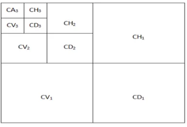
French mathematician Morlet J. et al. The wavelet transform has become a powerful signal processing tool based on Fourier transform, which has been developed and perfected by many scholars. Its theoretical basis is invariance under translation and extension, which allows the signal to be decomposed into sub-bands (time and frequency) without losing the information of the original signal [8]. According to the Mallat pyramid decomposition algorithm, the wavelet decomposition of two-dimensional image is realized quickly. After the wavelet decomposition of digital images, a series of sub-bands after decomposition is shown in Fig.1. In Fig.1, CAi is the low-frequency coefficient of layer i for wavelet decomposition. And the CHi, CVi and [image:3.612.100.293.492.623.2]CDi are the horizontal, vertical and the diagonal direction detail component of the i-layer after decomposition separately. [8]
Fig. 1 Schematic diagram of tertiarywavelet
To
understand the wavelet transform, let us recall the definition of convolution of a time function f (t) with a kernel g(t): [8]ψ t ∅ . t ∅ . t
√2
∅ 2t ∅ 2t 1 . . 1
And set
𝜓 , 𝑡 𝜓 𝑡 𝑛
𝜙 , 𝑡 𝜙 , 𝑡
√2
𝑓𝑜𝑟 𝑛 0 ,1 , . . 𝑁 1. … 2
Then the set 𝜓, is an orthonormal basis for
𝑤
, the orthogonal complement of𝑣
in𝑣
. Discrete wavelet transform : the space𝑣
can be decomposed as the orthogonal sum 𝑣 𝑣 ⊕ 𝑤 where𝑤
ai the orthogonal complement of𝑣
in𝑣
,and𝑣
therefore has the two bases𝜙 𝜙 , and 𝜙, 𝜓
𝜙 , , 𝜓 , ,3
The discrete wavelet transform (DWT) is the change of coordinates from
basis 𝜙 to the basis (𝜙, 𝜓 . if
g 𝑐 , , ∅, ∈ 𝑣 4
g 𝑐 , , ∅ , ∈ 𝑣 5
e 𝑤 , , 𝜓 , ∈ 𝑤 6
And 𝑔 𝑔 𝑒 then the DWT is given by [8]
𝑐 , 𝑐 , 𝑐 , /√2 … … … 7
𝑤 , 𝑐 , 𝑐 , /√2 … … … 8
3.2 Standard Deviation (STD)
After decomposing the images using Wavelet Transform, we can extract some important features using Mean, Standard Deviation. The mean is implemented as follows [9].
mean 1
5720 The Standard Deviation (STD) is implemented
as:[9]
STD ∑ ∑ f r, s mean
R S . . 10
3.3 HSV Color Space
HSV colour space represents colors in conditions of Hue (or colour-depth), Saturation (or colour-purity) and depth of the worthiness (or colour-brightness). Additionally it is known as HSB (Hue, Saturation, Brightness) or HSI (Hue, Saturation, Intensity). Hue identifies shade type, such as red, blue, or yellow. It requires worth from 0 to 360 (but it is normalized to 0-100% in a few applications). Saturation identifies the vibrancy or purity of the color. It takes values from 0 to 100%. Finally, Value aspect identifies the lighting of the color. It requires the same range as the saturation (0-100%). [10]
The conversion from RGB to HSV is defined by the following expressions (Eqs. (11), (12) ,(13),(14) and (15)) :
The R,G,B values are divided by 255 to change the range from [0-255] to [0-1]:
R R
255 , G G 255 , B
B
255 … … . 11
Cmax max R , G , B , Cmin
min R , G , B , Δ
Cmax – Cmin. . 12 Hue calculation:
H
⎩ ⎪ ⎨ ⎪
⎧60° ∆ mod 6 , if Cmax R′
60°
∆ 2 , if Cmax G
60°
∆ 4 , if Cmax B
.(13)
Saturation calculation:
S 0, if Cmax∆ 0
, if Cmax 0 100% ..(14)
Value calculation:
V Cmax) 100% .. .(15)
3.4 Grey Level Co-Occurrence Matrix (GLCM)
Using GLCM for extracting Gray various texture features. GLCM is also called as Gray level Dependency Matrix. It is defined as “A two dimensional histogram of gray levels for a pair of pixels, which are separated by a fixed spatial relationship.” GLCM of an image is computed using a displacement vector d, defined by its radius δ and orientation θ [11].
3.4.1 Energy:
This is a measure of local homogeneity in the image. Its value is high when the image has very good homogeneity. In a non-homogenous image, where there are many gray level transitions, the energy gets lower values. The measurement of energy is given by:[12]
𝐸𝑛𝑒𝑟𝑔𝑦 𝑝 𝑖, 𝑗 … 16
Where Ng is greatest level in gray level image, P (i,j) is GLCM matrix .
3.5 Watershed
In digital image handling, watershed is dependent on the three-dimensional image, and two will be the coordinate, another is grey level. Based on the idea of geography, there are three tips in the image: (1) Locality lowest point; (2) When a drop of water placed on the positioning of a point, the water must fall on a single minimum point. (3) Once the water reaches some point on the positioning, it will stream several such minimum amount point with the same likelihood. Then, for the least value of a specific region, the group of points which satisfy the condition (2) will be called the minimum amount "watershed" or "catchment basin",, and the set of points which satisfy the condition (3) and form together will be known as the "watershed." In the process of digital image, , the goal of the watershed algorithm [13] is to get the watershed and the watershed line in the image. [13] .
3.6 Fuzzy Logic
5721 than numeric values and can produce best results depend on indefinite verbal knowledge like humans. If a system’s behavior can be modelled by rules or requires very complex nonlinear processes, fuzzy logic can be applied to this system. Mamdani’s fuzzy inference method is the most commonly used fuzzy inference system. [14]
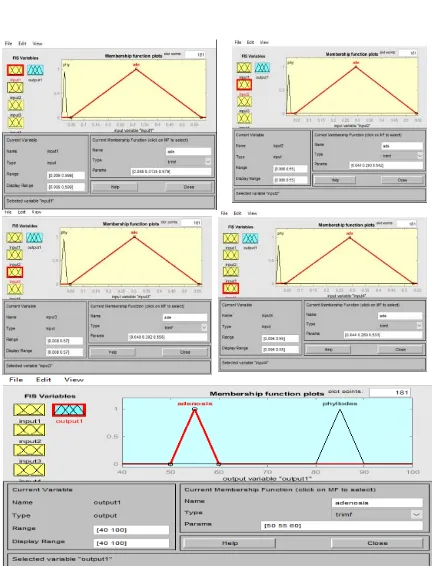
Fuzzy rule-based systems consist of three main steps; Fuzzification, Inference and Defuzzification. In the fuzzification step, the crisp input and output variables are defined and mapped to linguistics variables. Once the input and output variables and the corresponding membership functions are defined, a system of rules composed of IF-THEN statements is designed and the fuzzy inference takes place, producing a fuzzy output set. The output is then defuzzified during the defuzzification step to produce a crisp output value - the prediction . For our case, Range between (0-5) and (10-16) was used to represent the output which is the probability Malignant or Benign respectively [14]. And Range between (20-30) and (50-60) was used to represent the output which is one of the types of Benign breast cancer , And Range between (80-100) and (120-150) was used to represent the output which is one of the types of Malignant breast cancer .
4. THE PROPOSED ALGORITHM
Our proposed algorithm is consisting of six steps as shown in Figure 2
[image:5.612.311.519.192.384.2]
Figure 2 : The Algorithm flowchart
4.1 Step One Is Image Acquisitions:
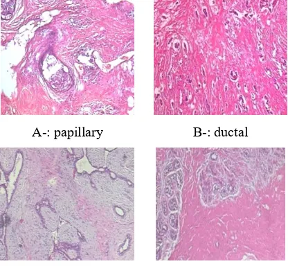
By collect the images database from internet (http://web.inf.ufpr.br/vr/breast-cancer-database) which is contain more than 1000 images we used 120 for training (60 Benign images and 60 Malignant images) , and 40 image for testing.as shown in Figure 3.
A-: papillary B-: ductal
C-: phyllodes_tumor D-: adenosis
Figure 3: (A and B) Malignant images , ( C and D) Benign images
4.2 Step Two Is Pre-Processing:
1. the pre-processing is starting by transform a histology colour image into grey scale image ; where the color image contain matrix with three color values for each pixel; Red (R), Green (G) and Blue (B), as shown in in Figure 4.
[image:5.612.77.302.461.722.2]
Figure 4: transform a histology image to grey scale image
2. stores all numeric variables as double-precision floating-point values that are 8 bytes (64 bits). These variables have data type (class) double. as shown in algorithm 1.
papillary ductal
Preprocessing
Diagnosis
adenosis phyllodes
Preprocessing
Diagnosis
Diagnosis
benign malignant
Input image
Preprocessing
5722
algorithm 1: Preprocessing
input: original image
output: enhanced image
step1: convert original image into gray scale
𝚼 𝟎. 𝟐𝟗𝟗𝐑 𝟎. 𝟓𝟖𝟕𝐆 𝟎. 𝟏𝟏𝟒𝐁. 𝟏𝟕
step2: convert resulted image into double image
End
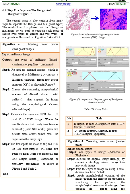
4.3 Step Three Is Feature Extraction :
1. Calculate CA1,CA2, CD2 and CA3 (the approximately parts of HWT for three levels respectively ); as shown in Figure.5.
[image:6.612.84.520.226.682.2]
Figure 5: HWT for three levels
2. Calculate STD1, STD2 , STD3 and STD4 for CA1, CA2 , CD2 and CA3 respectively. There are four features will obtained (std1, std2, std3, and std4) which be the inputs for the fuzzy logic, as shown in algorithm 2.
Algorithm 2 : Image Analysis
Input: gray image
Output: features extraction
Step1: Finding Haar wavelet to three level .(HWT)
Step2: Calculate CA1, CA2 , CD2 and CA3 for
three levels.
Step3: Calculate STD1, STD2 , STD3 and STD4
for step2 respectively. End
4.4 Step Four Is Diagnosis :
The objective of diagnosis step is to distinguish between malignant and benign melanoma, after obtaining features vector. In our algorithm , fuzzy logic is used for distinguishing between malignant and benign breast cancer (B.C.) in First phases , Algorithm (3.3) describes the steps diagnosis As shown in Figure 12.
Algorithm 3 : Diagnosis
Input: Features vector
Output: type of cancer (benign or malignant )
Step1: four input fuzzy logic will be the
features vector(STD1, STD2 and STD3 and STD4).
Step 2: build fuzzy logic ( two rules) , as shown in Figure 6 and Table 1.
Step3: one output form fuzzy logic (Benign or
Malignant) .
Table 1: Fuzzy Rules
No Rule
1 IF (input1 is duc+pap) OR (input2 is duc) OR
(input3 is duc_+_pap) OR (input4 is duc_+pap) THEN (output1 is B)
2 IF (input1 is ade_+phy) OR (input2 is ade+phy) OR
(input3 is ade_+_phy) OR (input4 is ade_+_phy) THEN (output1 is A)
5723
4.5 Step Five Separate The Benign And
Malignant Types :
The second stage is also contain from many steps to separate the Benign and Malignant types; The results from first phases will be Benign or malignant, so we need to separate each types of cancer (two types of Benign and two types of malignant) as illustrated in Algorithm 3.4 and 3.5
Algorithm 4 : Detecting breast cancer
(malignant image)
Input: malignant image
Output: one types of malignant (ductal_
carcinoma or papillary_ carcinoma)
Step1: Re-read the original image( which is
diagnosed as Malignant ) by convert a histology coloured image into colour moment (HSV) as shown in Figure 7
Step2: Creates the structuring morphological
element of discoid shape with radius=1 , then expands the image using the morphological element (discoid shape).
Step3: Calculate the mean and STD for H, S
and V of HSV image. Where the results shows that only two features mean of (H) and STD of (H) gives best results from others which will be inputs into the fuzzy logic .
Step4: The two inputs are mean of (H) and STD
of (H)) from (step 3) will build two rules of fuzzy logic for diagnosis and one output (ductal_ carcinoma or papillary_ carcinoma). as shown in Figure 8 and Table 2.
End
Figure 7: transform a histology image to color moment (HSV) image
Figure (8): Inputs and Outputs types of Malignant Mamdani model
Table (2): Fuzzy Rules
No Rule
1 IF (input1 is duc) OR (input2 is duc) THEN (output1 is ductal)
2 IF (input1 is pap) OR (input2 is pap) THEN (output1 is papulary)
Algorithm 5 : Detecting breast cancer (benign
image)
Input: benign image
Output: one types of benign (Adenosis or
Phyllodes)
Step1: Re-read the original image (Benign) by
convert a histology colour image into grey scale image.
Step2: Find the edges of image by using a
two-dimensional filter 'sobel' .
Step3: Apply morphological opening of the
[image:7.612.82.535.64.740.2] [image:7.612.305.534.222.388.2]5724 morphological element (discoid shape) .
Step4: Find the image complement and extracts
the regional maximums , then dilation to avoid marker and fragmentation removes smaller 5-pixel markers from the image.
Step5:convert image into binary then find the
watershed algorithm by final the boundaries of the marker. Which will convert the binary Colour watershed label image, as shown in figure (9,10).
Step6: apply GLCM onto grey scale image the
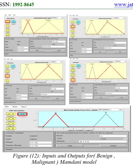
resulting of previous operations after histogram implementation on image . There are 16 features from GLCM these 16 features will build 16 rules of fuzzy logic and there are only one output (adenosis or phyllodes_tumor) as shown in Figure (11) and Table (3).
End
Figure (9): watershed operations part2
[image:8.612.315.531.88.371.2] [image:8.612.92.279.518.634.2]5725 Figure (11): Inputs and Outputs for( Benign , Malignant ) Mamdani model
Figure (12): Inputs and Outputs for( Benign , Malignant ) Mamdani model
No Rule
1 IF (input1 is ade) OR (input2 is ade) OR (input3
is ade) OR (input4 is ade) THEN (output1 is adenosis)
2 IF (input1 is phy) OR (input2 is phy) OR
(input3 is phy) OR (input4 is phy) THEN (output1 is phyllodes)
Table (3): Fuzzy Rules
5. RESULTS
In this section, we discus several concepts needed for our new algorithm . In This paper we use histopathology images for diagnosis the breast cancer through check the images if it is Benign (BC) or Malignant (BC) then classify each types of Benign with two types (adenosis and phyllodes_tumor) and Malignant with two types also (ductal_carcinoma and papillary_carcinoma). by use wavelet transform algorithm in first two steps of our algorithm then use GLCM and colour moment(HSV) in step three to the end, the features extracting for each step will be input to fuzzy logic to know the final decision, there are four features used as four inputs of fuzzy logic which give the final results (Benign or malignant) in first two steps and there are six features used as six inputs by calculate (MEAN , STD) for (H)of colour moment (H, S, V) for diagnosis the two types of Malignant and (energy (𝐴0°), energy
(𝐴45°) , energy 𝐴90°), energy (𝐴135°) ) for diagnosis the two types of Benign.
There four features in step two ( classify Benign and Malignant )which calculate by STD1, STD2 , STD3 and STD4 for CA1 , CA2 , CD2and CA3 of three levels WT respectively , as shown in Table (4 and 5). There are six features from steps three as shown in table (6 , 7 , 8 and 9)
Table (4).STD For Benign
Image No.
STD1 CA1
STD2 CA2
STD3 CA3
STD4 CD2
1 43.63146 81.3981 144.2333 8.366293
2 37.67848 69.13245 118.6775 8.067114
3 35.47462 66.36621 117.4697 6.592461
4 37.28117 70.91358 128.7396 6.059023
5 37.75304 70.2219 122.6454 7.511251
6 40.72568 75.18213 128.9053 8.678011
7 40.92783 75.20538 129.4749 9.10601
8 38.8137 71.01208 120.7492 8.928726
9 38.97185 71.32115 122.0768 9.014804
[image:9.612.95.308.71.336.2]10 39.36198 71.96632 121.364 9.09672
Figure 13 : Benign
Table (5). STD For Malignant
Image No.
STD1
CA1 STD2 CA2 STD3 CA3 STD4 CD2
1 99.56281 184.3522 319.3109 22.30879
2 98.53386 179.1271 302.6923 24.91326
3 90.35643 157.2049 243.9512 28.12394
4 91.66428 165.576 279.0232 24.82369
5 92.89925 164.9793 264.8339 25.65492
6 59.85532 107.7856 181.6433 16.2245
7 67.52448 124.2312 219.1201 16.09513
8 73.81036 141.7642 266.9144 12.50924
9 69.40446 120.1879 190.222 22.51926
10 92.65795 173.5048 315.3208 20.23946
[image:9.612.83.537.72.524.2] [image:9.612.316.530.217.489.2] [image:9.612.315.526.524.666.2]5726 Figure 14 : ma lignant
Table (6). (mean2 (H), STD (H)) For malignant(ductal_carcinoma)
Image No. mean2 (H) STD (H)
1 0.896701 0.031082
2 0.878165 0.044246
3 0.906455 0.006081
4 0.909259 0.042167
5 0.917552 0.026798
6 0.891837 0.003962
7 0.907903 0.006694
8 0.905304 0.007464
9 0.907001 0.020096
10 0.908558 0.013844
[image:10.612.93.532.51.198.2]
Figure 15 : ductal_carcinoma
Table (7). (mean2 (H), STD (H)) For Malignant (papillary_carcinoma)
Image No. mean2 (H) STD (H)
1 0.8581105 0.0971186
2 0.8137186 0.1216032
3 0.7814398 0.1422598
4 0.8420075 0.1145205
5 0.700039 0.0810016
6 0.7695641 0.1642349
7 0.6943092 0.1252418
8 0.8012199 0.1203206
9 0.8214097 0.1551491
10 0.7621288 0.1175079
Figure 16 : papillary_carcinoma
Table (8).STD For Benign(adenosis)
Image No.
Energy a1
Energy a2
Energy a3
Energy a4
1 0.31564 0.30764 0.320645 0.307528
2 0.38988 0.38103 0.394251 0.380613
3 0.38984 0.38076 0.39351 0.379236
4 0.29501 0.28767 0.299229 0.286296
5 0.54998 0.54262 0.556284 0.533915
6 0.49371 0.48345 0.502557 0.479568
7 0.4282 0.41964 0.429567 0.418053
8 0.16577 0.16149 0.168277 0.160703
9 0.23156 0.22813 0.23333 0.225815
10 0.48737 0.48089 0.491402 0.476215
Figure 17 : Benign(adenosis)
Table (9).STD For Benign(phyllodes_tumor)
Image No.
Energy
a1 Energy a2 Energy a3 Energy a4
1 0.01264 0.00924 0.01233 0.01024
2 0.01409 0.01012 0.01304 0.01098
3 0.01285 0.00822 0.01087 0.00836
4 0.01446 0.01088 0.0125 0.01002
5 0.01337 0.0102 0.01199 0.00896
6 0.01308 0.00993 0.01219 0.00952
7 0.01428 0.01164 0.01374 0.01105
8 0.01301 0.0111 0.01463 0.01092
9 0.01262 0.01076 0.0142 0.01057
[image:10.612.86.539.61.628.2] [image:10.612.84.291.236.471.2] [image:10.612.309.540.252.529.2] [image:10.612.308.536.576.716.2]5727 Figure 18 : Benign(phyllodes_tumor)
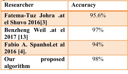
6. COMPRESSION OUR ALGORITHM
WITH OTHERS
There are many researches in diagnosis Breast cancer or detection , so that there are difference result and difference accuracy of researches . Table.10 shows the difference between our proposed algorithm with other researches algorithms.
Researcher Accuracy
Fatema-Tuz Johra .at
el Shuvo 2016[3] 95.6%
Benzheng Weil .at el
2017 [13] 97%
Fabio A. Spanhol.et al
2016 [4]. 94%
Our proposed
algorithm 98%
7. CONCLUSION
It is important to work in the field of early detection of breast cancer by using histological images because of the multiplicity of devices used in obtaining histological images and their accuracy, in addition to the distortions that occur during the conservation and storage phase of microscopic microscopy. Through the proposed algorithm and the conclusions reached, we recall the following conclusions:
1. In our algorithm we used Discrete Wavelet Transform with three levels each level has four parts, the total number of parts are 12 separate parts; (CA1 , CH1 , CV1, CD1 , CA2 , CH2 , CV2 , CD2 , CA3 , CH3 , CV3 and CD3) but the experiments shows that CA1 , CA2 , CD2 and CA3 are the best parts will give the best feature for diagnosis whither the cancer is Benign or malignant.
2. For recognition and diagnosis the two types of Malignant based on color features in general, the color model (HSV) that led to higher recognition results in color images. through used colour moment for each part of HSV ( H, S, V respectively), and calculate (Mean , STD) for each part (H, S, V respectively), will collect six features (Mean for H , STD for H, Mean for S , STD for S, Mean for V , STD for V) but the experiments shows that (Mean for H and STD for H) give the best features to diagnosis the two types of Malignant.
3. For recognition and diagnosis the two types of Benign Brest cancer based on GLCM with 16 features Distributed by using (contrast , energy , correlation , homogeneity in 0°, 45°, 90°, 135) but the experiments shows that (energy (in 0°), energy (in 45°) , energy in 90°), energy (in 135°) ) are the best ones which give the best features for diagnosis the two types of Benign.
4. Different kinds of statistical features are used such as Entropy, Mean, Moment and Standard Deviation but the experiments shows that the best ones are STD , Energy and Mean .
5. We hope that work can lead to more specialized medical decision support systems to help the patients to discover malignant and benign Breast Tumor in early cases. As such, we have identified several areas of future work that would benefit the breast cancer detection researches:
a) The improvement of the suggested online breast tumor recognition system to build self-detection system for the patients.
b) Use the same technique to diagnose other types of breast cancer using histological images. c) Experience this technique in categorizing other
tissue images for other types of cancers (not only Breast cancer).
d) This technique is used the same types of images but with different scale of the microscope zoom (2X, 6X, 10X, 15X, ….etc.) used to visualize the tissue.
REFERENCES:
5728 [2] M. Oussama and M. A. Kh, "Guidelines for
the early detection and screening of breast cancer," World Health Organization, pp. 24-6, 2006.
[3] F.-T. Johra and M. M. H. Shuvo, "Detection of breast cancer from histopathology image and classifying benign and malignant state using fuzzy logic," in Electrical Engineering and Information Communication Technology (ICEEICT), 2016 3rd International Conference on, 2016, pp. 1-5.
[4] F. A. Spanhol, L. S. Oliveira, C. Petitjean, and L. Heutte, "A dataset for breast cancer histopathological image classification," IEEE Transactions on Biomedical Engineering, vol. 63, pp. 1455-1462, 2016.
[5] M. Veta, J. P. Pluim, P. J. Van Diest, and M. A. Viergever, "Breast cancer histopathology image analysis: A review," IEEE Transactions on Biomedical Engineering, vol. 61, pp. 1400-1411, 2014.
[6] M. Al-Ayyoub, S. M. AlZu'bi, Y. Jararweh, and M. A. Alsmirat, "A GPU-based breast cancer detection system using Single Pass Fuzzy C-Means clustering algorithm," in Multimedia Computing and Systems (ICMCS), 2016 5th International Conference on, 2016, pp. 650-654.
[7] F. S. Ahadi, M. R. Desai, C. Lei, Y. Li, and R. Jia, "Feature-Based classification and diagnosis of breast cancer using fuzzy inference system," in Information and Automation (ICIA), 2017 IEEE International Conference on, 2017, pp. 517-522.
[8] X. Xinyu, W. Guoxin, Z. Chunmei, G. Qiaoman, and D. Chunyan, "Image enhancement algorithm of Dongba manuscripts based on wavelet analysis and grey relational theory," in Electronic Measurement & Instruments (ICEMI), 2017 13th IEEE International Conference on, 2017, pp. 340-345.
[9] R. K. Thakur and C. Saravanan, "Classification of color hazy images," in Electrical, Electronics, and Optimization Techniques (ICEEOT), International Conference on, 2016, pp. 2159-2163.
[10] J. M. Chaves-González, M. A. Vega-Rodríguez, J. A. Gómez-Pulido, and J. M. Sánchez-Pérez, "Detecting skin in face recognition systems: A colour spaces study," Digital Signal Processing, vol. 20, pp. 806-823, 2010.
[11] M. Alabed, "A Novel approach in the Detection of Obstructive sleep apnea from electrocardiogram signals using neural network classification of textural features extracted from time-frequency plots," 2007. [12] A. H. H. AlAsadi and B. M. R. AL-Safy,
Early detection and classification of melanoma skin cancer: LAP LAMBERT Academic Publishing, 2016.
[13] J. Gao, J. Dai, and P. Zhang, "Region-based Moving Shadow Detection Using Watershed Algorithm," in Computer, Consumer and Control (IS3C), 2016 International Symposium on, 2016, pp. 846-849.