NUMERICAL ANALYSIS OF THE BOUDARY EFFECT OF RADIAL
BASIS FUNCTIONS IN 3D SURFACE RECONSTRUCTION
Xiangchao Zhang, Xiangqian Jiang and Andrew Crampton
Centre for Precision Technologies, University of Huddersfield, Huddersfield, HD1 3DH, UK
ABSTRACT
Surface reconstruction is very important for surface characterization and graph processing. Radial basis function has now become a popular method to reconstruct 3D surfaces from scattered data. However, it is relatively inaccurate at the boundary region. To solve this problem, a circle of new centres are added outside the domain of interest. The factors that influence the boundary behaviour are analyzed quantitatively via numerical experiments. It is demonstrated that if the new centres are properly located, the boundary problem can be effectively overcome whilst not reducing the accuracy at the interior area. A modified Graham scan technique is employed to obtain the boundary points from a scattered point set. These boundary points are extended outside with an appropriate distance, and then uniformized to form the new auxiliary centres.
Keywords Surface reconstruction, Boundary effect, Radial basis function, Centre treatment
1 Introduction
In the precision metrology field, data can be classified into discrete data and continuous data. In practice, the measurement data are usually obtained from physical objects via coordinate measurement machine, laser scanning etc, and consequently are in discrete form. The surface information between the measurement data points is sometimes required. Therefore it is necessary to get a continuous representation from these discrete data. Surface reconstruction (also termed surface
fitting or modelling) is to obtain a continuous surface Q that best explains the given discrete point set P,
i.e. to minimize the difference between them under some error criterion, e.g. using the ordinary least squares,
∑
=− = N
i
i i
i f x y
z E
1
2 )] , (
[ (1) In the equation,
z
=
f
(
x
,
y
)
is the unknown function representation of Q andP
i=
T i i i
y
z
x
,
,
]
[
,i
=
1
,...,
N
is an arbitrary point of the measurement data P.Radial basis function (RBF) method is now very extensively used for multivariate scattered node interpolation [1,2]. Given an arbitrary point d
R
∈
x
, this method selects certain fixed centres {cj},d j
∈
R
c
, j=1,…, M. A radial basis function is defined as,) ( ) (
)
( j j
j =
φ
− =φ
rΦ x x c (2) where
r
j=
x
−
c
j denotes the Euclidian distance.Therefore the function value f associated with the point x can be represented as,
∑
=
−
=
Mj
j j
w
f
1
)
(
)
(
x
φ
x
c
(3) where {wj} are weighting parameters.2. Boundary Problem of RBF Reconstruction
2.1. Problem Statement and Related Work
The surface used in precision metrology is usually an open surface patch. The fitting accuracy near the boundary will be degraded compared with the interior area. For surfaces sufficiently smooth, the accuracy in the interior region can attain O(h4) for the basis function of thin plate splines, while at the boundary it is not better than O(h5/2) in the sense of L-2 norm. Here the fill distance h measures the
data density [3]. This effect severely limits the application of the RBF method, especially when the boundary information is of our particular interest. To the best knowledge of the authors, very few researchers paid attention to this problem and nearly all the proposed approaches deal with this problem by changing the arrangement of the boundary centres. Hangelbroek [3] analyzed the boundary effect theoretically and proposed using an increased centre density at the boundary region. Fedoseyev [4] deployed some additional centres outside the domain of interest to mitigate the boundary problem of partial differential equations. Fornberg [5] observed the boundary effect via several numerical examples and suggested moving the boundary centres outside. However, the relationship between the fitting accuracy and the centre density and/or moving distance is not clearly indicated. In this paper, some numerical experiments will be presented and the factors which influence the boundary behaviour will be studied systematically.
2.2. Comparison of Some Common Boundary Treatments
The condition numbers of infinitely smooth basis functions like Gaussian, multiquadric etc are terribly large compared to non-smooth basis functions like TPS [6]. Additionally, their scaling is a crucial issue for accuracy and stability. To concentrate on the influence of the centre distribution, we adopt the thin plate spline as basis function, which contains no shape parameters and thus is scale invariant. To investigate the behaviours of RBF in different situations, we select six typical smooth functions as test surfaces [7], as illustrated in Figure 1.
The data points are sampled uniformly from the domain with spacing
h=0.035. The centres are also uniformly selected within the domain. For the linear system in Equation (2), weighting parameters are to be calculated. To make the function uniquely solvable, the number of centres should not exceed that of the data points. Consequently the centres are sampled with a greater spacing H=0.05. The equation is solved in the sense of L-2 norm which minimizes the summation the squared residuals at the evaluation locations. RBF method usually has high accuracy at the data positions and oscillates between them, which is known as the over-fitting problem [8]. Thus the residuals at the data positions cannot completely reflect the reconstruction quality. Hence we sample evaluation points within the domain of interest with a spacing h1=0.015. The reconstruction error with
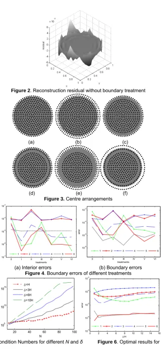
respect to the ideal test surface is illuminated in Figure 2. It is evident that severe error appears at the boundary. To investigate the boundary effect quantitatively, the boundary region is defined as the narrow annular region with a width w=0.15 according to the experimental results. The fitting errors at the interior and outer areas are evaluated separately.
25 . 0 ) 5 . 0 ( ) 5 . 0
(x− 2 + y− 2 ≤
Some common boundary treatments are listed below:
(I) Adding one circle of centres outside the domain of interest; (II) Adding two circles of centres outside the domain of interest;
(III) Moving the outmost one circle of centres outside with a distance
δ
=H; (IV) Moving the outmost two circles of centres together with a distanceδ
=H; (V) Moving the outmost two circles of centres together with a distanceδ
=2H and (VI) Moving the outmost two circles with distancesδ
1=2H andδ
2=H respectively;In all these six cases, the centres remain quasi-uniform, i.e. the centre spacing in the interior domain and at the boundary is kept to be H. Their centre arrangements are illustrated in Figure 3(a)-(f) respectively. The corresponding condition numbers (Cond) of the interpolation matrices are listed in Table 1. For comparison, the case without boundary treatment is called Case 0. It can be seen that all the six condition numbers are larger than Case 0, especially Case 2, consequently the numerical stability is degraded. To make the solutions trustworthy, Truncated Singular Value Decomposition is applied for Cases II and V, and QR decomposition for other cases [9].
We calculated the Sa (mean absolute deviation), Sq (root mean squared error) and St (max-min error) for the interior and boundary areas respectively, and found these three error metrics show very similar behaviours. Consequently only Sq values are presented here, see Figure 4. Note that Case II spoils the fitting quality both in the interior and the boundary areas of Surfaces 2 and 3. For other surfaces, the improvement is not significant. Considering its ill-conditioning property, this technique will not be adopted. Case III can retain the interior accuracy, but its boundary performance depends heavily on the surface shape, thus not very reliable. Cases IV and V are termed ‘Not-a-Knot’ and ‘Super
Not-a-Knot’ respectively by Fornberg et al [5]. Unlike their conclusions, moving boundary centres outside as
Furthermore, Case V is not always better than IV. Case VI takes very similar effect with IV except for obtaining better result for Surface 1. On the contrary, Case I can greatly improve the fitting accuracy both in the inner and outer areas of all the six test surfaces. It is proved to be the most reliable method. Hence we adopt this technique for boundary improvement. A phenomenon worth noting is that the error at the central region of Surface V remains nearly constant. This is due to its shape―― it has a very planar boundary. For Surfaces 2, 3 and 6 which have steep boundary regions, the inner accuracy is improved by at least one order. That is to say, the influence of boundary enhancement techniques on the inner area is in positive correlation with the slope of the boundary region.
2.3. The Factors Influencing the Boundary Behaviour
Among the six treatments, adding one circle of centres is thought to be an effective trick. Another superiority of this approach is its ease to implement compared with other treatments. In the previous section, the spacing and the distance of the added centres are fixed to be H. Consequently a question arises: what is the relationship between the fitting quality and the distribution of the added centres, such as the number N of the added centres and the distance
δ
from the boundary to the added circle? For each surface, we set the distanceδ
=H,3H,6H and 10H respectively and change the number Nfrom 12 to 100. The corresponding condition numbers are shown in Figure 5. With N and δ increasing, the condition number increases exponentially, consequently degrading the stability. Thus we adopt Truncated Singular Value Decomposition to solve the weighting parameters.
Now we change the distance δfrom H to 15H. For a fixed δ value, the point number N ranges from 12 to 120 and the optimal result among them is recorded. The final result is given in Figure 6. It can be seen that Surfaces 2, 4, and 5 achieve the best result at the interval
δ
∈[2H,4H]. Surfaces 3 and 6 prefer a smaller δ value andδ
=8H is the best choice for Surface 1. When δ is large enough, all thesix surfaces behave very steadily and stay nearly unchanged. Here only the influence of one factor δ is clarified. What is the effect of the point number N?
Again for each surface, we select
δ
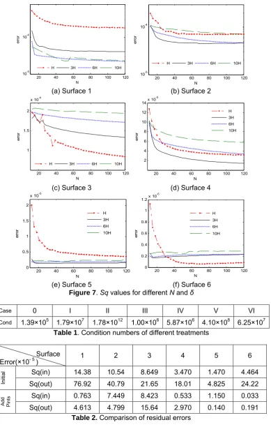
=H,3H,6H and 10H and change the point number N. The corresponding Sq curves are plotted in Figure 7. Whenδ
=H , Sq is very sensitive to the added point number N. A larger N is preferred for all test functions. With δ increasing, the reconstruction quality is less and less sensitive to N and differentiated by surface shapes. Therefore it is impossible to give an optimal δ and N which are always the best choice in all situations. Our purpose is to supply an approach which is effective and reliable for various surface shapes. Taking the numerical stability into account, we select δ=3H. The reconstruction result will enter steady region when N>40, therefore N=40 is adopted. In this case, the corresponding spacing between the added points isε
=2H .Table 2 lists the Sq (Root Mean Squared Error) for the initial Case 0 and the optimal boundary treatment which adds new centres with δ=3H and ε=2H. The error metrics are supplied for both the inner and outer regions. It is evident that this boundary treatment does improve the reconstruction performance. It can depress the boundary error whilst not reducing the accuracy at the interior area. The boundary accuracy improvement is highly related to the boundary shape. If the surface has a planar boundary curve with relatively small height variation, like Surfaces 5 and 6, the boundary performance can be significantly better. While for surfaces with very steep boundaries which jump greatly in height, like Surfaces 3 and 4, the improvement will not be so prominent. As for smooth surfaces with common shape, like Surfaces 1 and 2, the behaviour is medium. In a word, the effect of this technique is in negative correlation with the boundary height range. Thus for surfaces with planar boundary curves, it is an appropriate approach to add extra centres outside to improve the boundary accuracy. It is worth noting that Surface 3 has the least improvement both in the interior and outer areas among the six surfaces. This is caused by the severe shape asymmetry and distinct step. Fortunately, this kind of surface is very rare in practice.
3. Conclusions
RBF reconstruction behaves poorly at the boundary. To solve this problem, six centre treatments are compared quantitatively for different surface shapes. Adding one circle of new centres outside the domain of interest is found to be an effective approach. Numerical experiments are presented to analyze the relationship between the fitting quality and N (the number of the added centres) and
δ
(the distance from the added circle to the boundary). It is demonstrated that this technique can effectively overcome the boundary problem whilst not reducing the accuracy at the interior area,especially for surfaces which have planar boundary curves. As the numerical stability will be degraded exponentially with increasing δ and N, an appropriate composite is made. To obtain the boundary from an arbitrary discrete point set, a modified Graham scan algorithm is employed [10]. All the boundary points are moved outside to form a new circle, which are added as new centres for radial basis function reconstruction.
References
1. Hardy R.L. Multiquadric equation of topography and other irregular surfaces. J Geophysics
Research. 76: 1905-1915(1971)
2. Crampton A. Radial basis and support vector machine algorithms for approximating discrete data.
PhD Thesis. University of Huddersfield, UK(2002)
3. Hangelbroek T. Error estimates for thin plate spline approximation in the disc. ftp://ftp.cs.wisc.edu/Approx/TPSerror.pdf(2007)
4. Fedoseyev A.I., Friedman M.J. and Kansa E.J. Improved multiquadric method for elliptic partial differential equations via PDE collocation on the boundary. Computers and Mathematics with
Applications. 43: 439-455(2002)
5. Fornberg B., Driscoll T.A., Wright G. and Charles R. Observations on the behaviour of radial basis function approximations near boundaries. Comp and Math with Appl. 43: 473-490(2002)
6. Schaback R. Multivariate interpolation and approximation by translates of a basis function. In: Chui C.K, Schmaker L.L. (Eds), Approximation Theory VIII, 1: 491-514(1995)
7. Lee S, Wolberg G. and Shin S.Y. Scattered data interpolation with multilevel B-splines. IEEE Trans.
Visualization and Computer Graphics. 3(3): 1-17(1997)
8. Bishop C.M. Neural Networks for Pattern Recognition. Oxford University Press. (1995) 9. Björck Å. Numerical Methods for Least Squares Problems. SIAM(1996)
10. Graham R.L. An efficient algorithm for determining the convex hull of a finite planar set. Information
Processing Letters. 1: 73-82(1972)
(1) (2) (3)
(4) (5) (6)
Figure 1. Test Surfaces
Figure 2. Reconstruction residual without boundary treatment
(a) (b) (c)
(d) (e) (f)
Figure 3. Centre arrangements
0 I II III IV V VI
10-7
10-6 10-5
10-4
10-3
treatments
error
1 2 3 4 5 6
0 I II III IV V VI
10-6 10-5 10-4 10-3
treatments
erro
r
1 2 3 4 5 6
(a) Interior errors (b) Boundary errors
Figure 4. Boundary errors of different treatments
20 40 60 80 100
105 1010 1015
N
Con
d
δ=H δ=3H δ=6H δ=10H
0 2 4 6 8 10 12 14 16
10-7 10-6 10-5 10-4 10-3
δ/H
er
ror
[image:5.595.159.486.55.774.2]1 2 3 4 5 6
Figure 5. Condition Numbers for different N and δ Figure 6. Optimal results for different δ
6
20 40 60 80 100 120
10-5 10-4
N
erro
r
H 3H 6H 10H
20 40 60 80 100 120
10-5 10-4
N
erro
r
H 3H 6H 10H
(a) Surface 1 (b) Surface 2
20 40 60 80 100 120
1 1.5 2
x 10-4
N
error
H 3H 6H 10H
20 40 60 80 100 120
2 4 6 8 10 12 14x 10
-5
N
er
ror
H 3H 6H 10H
(c) Surface 3 (d) Surface 4
20 40 60 80 100 120
0 0.5 1 1.5 2
x 10-5
N
erro
r
H 3H 6H 10H
20 40 60 80 100 120
0 0.2 0.4 0.6 0.8 1 1.2x 10
-5
N
er
ro
r
H 3H 6H 10H
(e) Surface 5 (f) Surface 6
Figure 7. Sq values for different N and δ
Case 0 I II III IV V VI
Cond 1.39×10⁵ 1.79×10⁷ 1.78×10¹² 1.00×10⁶ 5.87×10⁶ 4.10×10⁸ 6.25×10⁷ Table 1. Condition numbers of different treatments
Surface
Error(×10- 5 ) 1 2 3 4 5 6
Initial
Sq(in) 14.38 10.54 8.649 3.470 1.470 4.464 Sq(out) 76.92 40.79 21.65 18.01 4.825 24.22
Add Pints
[image:6.595.129.519.75.688.2]Sq(in) 0.763 7.449 8.423 0.533 1.150 0.033 Sq(out) 4.613 4.799 15.64 2.970 0.140 0.191