Network Coding for Resource Optimization and Error Correction

(1)

Network coding for resource optimization and

error correction

Thesis by

Sukwon Kim

In Partial Fulfillment of the Requirements for the Degree of

Doctor of Philosophy

California Institute of Technology Pasadena, California

2010

(2)

c

° 2010

(3)

(4)

Acknowledgements

I would like to express my immense gratitude to my advisors, Professor Michelle Effros and Professor Tracey Ho for their support, guidance, and encouragement throughout the period of my graduate studies. I am very grateful that their constant passion, insight and curiosity leads me to memorable research experience. I have learned the most significant thing for the future of my life, the excitement of research, by working with them. I also give my deep gratitude to their kindness for frequent discussions and advices.

I would like to thank the members of my candidacy and defense committees, Pro-fessors Steven Low, Jehoshua Bruck, Michelle Effros, Tracey Ho, and Babak Hassibi, who read my thesis manuscript and gave me valuable feedback on my work. I also want to thank to Professor Salman Avestimehr for his consistent advice on network error correction.

I would like to give my deepest gratitude to my family. Their unconditional love and patience were the most significant support for my Ph.D abroad study. I thank my family for all the things they gave to me. I also wish to thank my friends Hyunsup Park, Jaeseok Bae, Kwanghyung Chung, Inmo Han, JunHwan Kim, Woojun Han, Keosan Kim, Christopher Chang, Changho Sohn, Hyungjoon Ahn, Minjang Jin, and Haekong Kim for their consistent encouragement.

(5)

(6)

Abstract

In the first part of this thesis, we demonstrate the benefits of network coding for optimizing the use of various network resources.

We first study the problem of minimizing the power consumption for wireless multiple unicasts. A simple XOR-based coding strategy is considered for reducing the power consumption. We present a centralized polynomial time algorithm that approximately minimizes the number of transmissions for two unicast sessions. We extend it to a greedy algorithm for general problem of multiple unicasts.

Previous results on network coding for low-power wireless transmissions of mul-tiple unicasts rely on opportunistic coding or centralized optimization to reduce the power consumption. Thus we propose a distributed strategy for reducing the power consumption with wireless multiple unicasts. Our strategy attempts to increase net-work coding opportunities without the overhead required for centralized design or coordination. We present a polynomial time algorithm using our strategy that max-imizes the expected power savings with respect to the random choice of sources and sinks on the wireless rectangular grid.

We study the problem of minimum-energy multicast using network coding in mo-bile ad hoc networks (MANETs). The optimal subgraph can be obtained by solving a linear program every time slot, but it leads to high computational complexity. We present a low-complexity approach, network coding with periodic recomputation, which recomputes an approximate solution at fixed time intervals, and uses this solu-tion during each time interval. We analyze the power consumpsolu-tion and the complexity of network with this approach.

(7)

are presented for multiple unicasts and multicast. Such algorithms are distributed since decisions are made locally at each node based on feedback about the size of queues at the destination node of each link. We develop a back-pressure based dis-tributed optimization framework, which can be used for optimizing over any class of network codes. Our approach is to specify the class of coding operations by a set of generalized links, and to develop optimization tools that apply to any network composed of such generalized links.

(8)

List of Figures

1.1 Transmitting messages m1,3 and m3,1 from v1 to v3 and v3 to v1, re-spectively, requires three transmissions with network coding and four without. . . 2 1.2 3-star coding: si wants to transmit packet xi to ti (1 ≤ i ≤ 3) and tj

overhears from si (j 6=i). Node v broadcasts x1⊕x2⊕x3 to t1, t2, and

t3 and it gives a savings of two transmissions. . . 4 1.3 Point to point channel composed of n forward links andm feedback links. 9 1.4 Four node acyclic networks: unbounded reliable communication is

al-lowed from source S to its neighbor B on one side of the cut and from node A to sink U on the other side of the cut, respectively. There are feedback links from A toB. . . 9 1.5 k-layer zig-zag network: Ai and Bi can communicate reliably with

un-bounded rate to Ai+1 and Bi+1, respectively.(S = B0, U =Ak+1). The

links from Ai toBi represent feedback across the cut. This model more

accurately captures the behavior of any cut with kfeedback links across the cut. . . 10

2.1 The nodes of the network lie on the vertices of a triangular lattice. . . 11 2.2 Reverse carpooling. . . 12 2.3 Reverse carpooling solution of two unicast sessions with one reverse

car-pooling segment and four branches. . . 14 2.4 Illustration of cost of edge (v, v0_{): 5 unicasts use edge (v, v}0_{) and 4}

unicasts use edge (v0_{, v). Combined contribution of edges (v, v}0_{) and}

(11)

2.5 Reverse carpooling is possible at nodes a,b,c,and d in the first network. In the second network, reverse carpooling is not possible at nodesa, and d because t2 cannot overhear the transmission from s1 and t1 cannot overhear the transmission from s2. Thus the first network requires 6 transmissions, while the second network requires 8 transmissions. In both networks, we approximate the cost of S as C(S) = 7. In general, for a reverse carpooling segment ofnlinks shared by two unicast sessions, the actual number of transmissions is n±1 while the approximate cost is n. . . . 17 2.6 Illustration of a 4-exit loop and a 2-exit loop. . . 18 2.7 Illustration of proof of Theorem 2.2: (a) S∗ _{= (P1, P2, P3) contains a}

4-exit loop L(P1, P2, k, m). (b) Redirecting both P1 and P2 as shown removes rk(P1, P2) and rk+1(P1, P2) and decreases the cost of the solution. 20

2.8 Lemma 2.4 of Theorem 2.3. First portion of proof: If c is above ga,0, then gb,0 6∈4abc. If c is below gb,0, then ga,06∈4abc. If cis between ga,0 and gb,0, then ga,0, gb,0 6∈ 4abc. . . . 22 2.9 Case 1 of Theorem 2.3: ∠a,∠b,∠ccontain one gridline respectively,ga,60,

gb,0, and gc,120. These grid lines form an equilateral triangle 4uvw. . . 23 2.10 Case 1 of Theorem 2.3: Any point outside of the triangle uvw cannot

be a solution. . . 25 2.11 Case 1 of Theorem 2.3: Any point outside of the triangle uvw cannot

be a solution. . . 25 2.12 Case 2 of Theorem 2.3: ∠a contains three grid lines. a is the unique

solution point. . . 26 2.13 Reverse carpooling solution S(b, c). . . . 27 2.14 Each angle in 4bs2t1 contains one grid line. . . 29 2.15 Simulation result: As the number of unicast sessions is increased,E(C(Sn)

Ln )

is decreased. . . 31 2.16 Simulation result: We extend the result in Fig. 2.8. When 100 unicast

sessions are chosen uniformly at random on the grid, E(C(Sn)

(12)

2.17 Case 2 in the calculation of edge use distributionr1_{(e). (a)}_h

i−1 ≤s1y <

hi and (b) hi < s1y < hi+1. . . 36 2.18 Case 4 in the calculation of r1_{(e). (a) 0} _≤ _s1

y < hi (j ≤ i) and (b)

hi ≤s1y ≤b and hi+1 ≤t1y ≤m. . . . 37

2.19 Case 5 in the calculation of r1_{(e). (a)} _h

i+1 ≤ s1y ≤ m (j ≥i+ 1) and

(b) b+ 1≤s1y < hi+1 and 0≤t1y < hi. . . 37

2.20 Given hk and hk+1, optimizing (h1, ..., ht) is equivalent to optimizing

(h1, .., hk−1) in (a) and (hk+2, .., ht) in (b). . . 39

2.21 Function lq(a, b, c, d) finds the optimal 2q+1−2 reverse carpooling lines

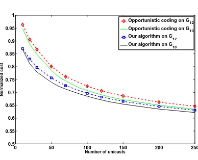
between two upper reverse carpooling lines at locations c and d and two lower reverse carpooling lines at locations a and b and returns its expected cost. . . 41 2.22 Normalized cost on G10 and G12. . . . 43 2.23 Case 2 in the path choice algorithm (a) when f > g and (b) when f < g. 44 2.24 Case 1 in the calculation of edge use distribution r1_{(e) when 0}_≤_s

1x <

rp. (a) s1y ≤t1y and (b) s1y > t1y. . . 45

2.25 (a) Case 1 in the calculation of edge use distribution r1_{(e) when} _r

p ≤

s1x ≤ a. (b) Case 2 in the calculation of edge use distribution r1(e)

when 0≤s1x < rp. . . 45

2.26 Case 4 in the calculation of edge use distribution r1_{(e) when}_{c < d} _and f < g. (a) hq+1 ≤t1y ≤m and (b)b+ 1≤t1y < hq+1. . . 47 2.27 Case 4 in the calculation of edge use distribution r1_{(e) when}_{c > d} _and

f < g. (a) 0≤s1y < hq and (b)hq ≤s1y ≤b. . . . 47

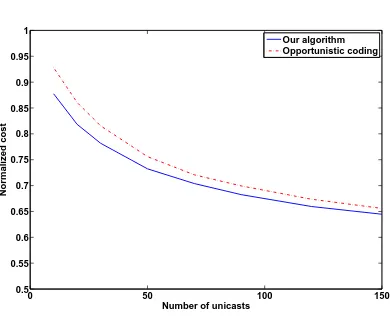
2.28 Case 5 in the calculation of edge use distribution r1_{(e) when}_c₆₌_d _and f 6=g (a) c < d and (b)c > d. . . . 48 2.29 Normalized cost on G8. . . 50 2.30 Scenario: 5 rooms are distributed over large area. Distance between any

(13)

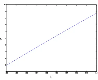
2.31 Optimal fractional performance gap at the start of the interval,r, versus R, an upper bound on the fractional optimality gap over each interval, when α= 10−3 _and _M _{= 1000. . . .} ₆₇ 2.32 Optimal length of interval, p∗_{, versus} _R _when _α_{= 10}−3 _and _M _{= 1000.} ₆₇ 2.33 Reverse carpooling : (a) Transmitting messages m1,3 and m3,1 from

v1 to v3 and v3 to v1, respectively, requires three transmissions with network coding and four without. (b) Generalize reverse carpooling for two unicast sessions which overlap in opposite directions. . . 72 2.34 (a) 2-star coding : p1 and p2 want to transmit packets x1 and x2 to

m1 and m2 respectively. Since m2 overhears transmission from p1 and m1 overhears from p2, v transmits x1 ⊕x2 to m1 and m2. This saves a single transmission. (b) 3-star coding: si wants to transmit packet xi

to ti (1 ≤ i ≤ 3) and tj overhears from si (j 6= i). Node v broadcasts

x1⊕x2⊕x3 to t1, t2, and t3 and it gives a savings of two transmissions. 73 2.35 Pairwise XOR coding . . . 74 2.36 Backtracking approach: (a) Transmission pair (O,D) on the

general-ized link e where |O| = |D| = 1. Using the backtracking approach for this example, we move from Q1

d(t) to Q1o(t−T). (b) Transmission

pair (O,D) on the generalized link e where |O| = 2 and |D| = 1. Us-ing the backtrackUs-ing approach for this example, we move from Q1

d(t) to

max(Q1

o(t−T), Q2o(t−T)). . . 79

2.37 Example of case 2 in the proof of Lemma 2.14: we derive the maxi-mum length of queueWc0

k using our backtracking approach by following

(14)

3.1 Four-node acyclic network: unbounded reliable communication is al-lowed from source S to its neighbor B on one side of the cut and from node A to sink U on the other side of the cut, respectively. (a) There are 2 links of the capacity 10 fromS toAand 4 unit-capacity links from B to U. (b) There are 5 links of the capacity 3 from S toA. There are 2 links of the capacity 2 and 3 links of the capacity 1 from B toU. . . 100 3.2 2-layer zig-zag network: unbounded reliable communication is allowed

fromS toB, from B toD, from A toC, and from C to U respectively. There is a sufficiently large number of feedback links fromAtoB. There is one feedback link from C toD. . . 101 3.3 Four node acyclic network: There are 4 links of the capacity 2 from S

to A. There are 3 links of the capacity 2 and 1 link of the capacity 4 from B toU. . . 103 3.4 A single source and a single sink network: all links on the top layer have

capacity 2. All links on the middle and bottom layer have capacity 1. Whenz = 1, the capacity of this network is 2 while linear network codes achieve at most 4/3. . . 106 3.5 A single source and a single sink network: the link capacity in this

network is as follows: r(l1) = r(l2) = r(l3) = r(l4) = 4, r(l5) = ... = r(l10) = 2. All the links in the middle layer have capacity 1. Error correction at Y3 and Y4 is necessary for achieving the capacity. . . 111 3.6 A single source and a single sink network: all links on the top or middle

(15)

3.7 Four node acyclic networks: this network consists of 3 links of capacity 2 from S to A, 5 links of capacity 1 from B to U, 1 link of capacity 6 from A to B. Given the cut ({S, B},{A, U}), unbounded reliable communication is allowed from source S to its neighbor B on one side of the cut and from node A to sink U on the other side of the cut, respectively. . . 116 3.8 two-node network G with n forward links and m feedback links. . . 119 3.9 Four node acyclic networks: unbounded reliable communication is

al-lowed from source S to its neighbor B and from node A to sink U, respectively. This network consists of a links of arbitrary capacity from S to A, b links of arbitrary capacity from B to U. From A to B, there are m feedback links and each feedback link has the minimum capacity. 122 3.10 Four node acyclic networks: (a) z = 2 and feedback link transmits

(a1 +a2, b1+b2, c1 +c2). (b) z = 3. Assume that (a1, .., a6), (b1, .., b6), (c1, .., c4), (d1, .., d4), and (e1, e2, e3) are transmitted on forward links (l1, .., l5) from S to A, respectively. Feedback link also transmits the sum of codewords on each forward link. . . 124 3.11 k-layer zig-zag network: given the cutcut({S, B1, .., Bk},{A1, .., Ak, U}),

Ai and Bi can communicate reliably with unbounded rate to Ai+1 and Bi+1, respectively. (S = B0, U = Ak+1). The links from Ai to Bi

represent feedback across the cut. This model more accurately captures the behavior of any cut with k feedback links across the cut. . . 128 3.12 Reduced zig-zag networkG0_{such that}_m

(16)

List of Tables

(17)

Chapter 1

Introduction

A new paradigm for operating a network, network coding was first introduced Ahlswede et al. in paper [1],which generalizes traditional routing by allowing each node to per-form arbitrary operations on its inputs to generate the node’s output. It was shown that the capacity of the network is equal to the size of the minimum cut that sep-arates the source and any terminal. In a subsequent work, Li et al. [2] proved that linear network codes are sufficient to achieve the capacity of the network. An al-gebraic framework for linear network codes on directed graphs was developed by Koetter and Medard [3]. This framework was used by Ho et al. [4, 5] to construct random distributed network coding, which achieves the network capacity with prob-ability exponentially approaching 1 with the code length. Jaggi et al. [6] proposed a polynomial-time algorithm for systematically finding feasible network codes. Oppor-tunistic XOR coding, which allows coding between packets across different sessions, is proposed in [7].

(18)

Sev-- ¾

¾

-v1 v2 v3

v1 v2 v3

m1,3 m3,1

m1,3⊕m3,1

Figure 1.1: Transmitting messages m1,3 and m3,1 from v1 to v3 and v3 to v1, respec-tively, requires three transmissions with network coding and four without.

eral polynomial time algorithms are presented that minimize the power consumption in wireless networks with network coding. In [13,14], different optimization trade-offs in wireless networks with network coding are studied.

In Chapter 2, we demonstrate the benefits of network coding for optimizing the use of various network resources and propose several optimization algorithms.

(19)

Since both nodes v1 and v3 are within transmission range of node v2, both receive the mixture packet (m1,3⊕m3,1). Node v1 decodes m3,1 by taking the binary sum of m1,3 ⊕m3,1 and its known value of m1,3. Node v3 similarly knows m3,1 and receives m1,3 ⊕m3,1, from which it can decode m1,3. The given strategy generalizes from single packet transmissions across a two-hop network to information flows across a path with arbitrarily many hops. We call this strategy reverse carpooling. We use the word “carpooling” because the method allows two messages to effectively share a ride through the network: after an initial set-up period, every time an internal node transmits, it transmits a bit-wise binary sum of the next packet that it intends to send forward and the next packet that it intends to send backward along the path. For long paths and long sequences of packets the savings approaches a factor of two. We call it “reverse” carpooling because the strategy only applies when the informa-tion flows that want to share a ride are traveling opposite direcinforma-tions. In addiinforma-tion to the reverse carpooling advantage, network coding is useful at network crossroads, such as the bottleneck of the wireless butterfly example of [15] or other scenarios where overheard information may provide opportunities for coding [16]. An example of particular interest is shown in Fig. 1.2. Here a single packet (x1,4) passes from node v1 to node v4, another (x3,6) from node v3 to node v6, and a third (x5,2) from node v5 to node v2, The routing solution requires a minimum of six transmissions as each node transmits its known packet to node v7, which then sends each message along separately. In the network coding solution, here called 3-star coding, nodev7 finds the bit-wise binary sum x1,4 ⊕x3,6⊕x5,2 and sends that value to all three receivers in a single broadcast transmission. In this case, node v2 overhears node v1’s transmission of x1,4 simply because it is one of v1’s neighbors; it likewise overhears x3,6 due to its proximity to v3. Node v2 can therefore combine its overheard messages with the coded packet x1,4⊕x3,6 ⊕x5,2 to decode the desired message x5,2. Nodes v4 and v5 likewise overhear the messages that don’t interest them and use those to decode their desired packets from x1,4⊕x5,2⊕x3,6.

(20)

U ¸¾

s1 t3

s2 t2

s3 t1

v

¸

U ¾

s1 t3

s2 t2

s3 t1

v

Figure 1.2: 3-star coding: si wants to transmit packet xi to ti (1 ≤ i ≤ 3) and tj

overhears fromsi (j 6=i). Nodev broadcastsx1⊕x2⊕x3 tot1,t2, and t3 and it gives

a savings of two transmissions.

configuration allows each of the intersection outputs to overhear the message that it doesn’t require. Consider k different session’s packets p1, p2,..,pk at a node v that

have distinct next-hop nodes v1,..,vk respectively. For each next-hop node vi, if it is

the previous-hop node of packet pj or it overheard packet pj from the transmission

of its previous-hop node from opportunistic listening for ∀j 6= i, coded packet p = p1 ⊕ p2 ⊕. . .⊕ pk is broadcast to all the next-hop nodes v1,..,vk at node v. The

savings from such a crossing, here called ak-star, isk−1 transmissions. The wireless butterfly network of [15] is one such example. The savings from such a crossing, here called a 2-star, is a single transmission.

(21)

spent on reverse carpooling lines. Intermediate nodes apply reverse carpooling op-portunistically along these routes. Our network optimization attempts to choose the reverse carpooling lines in a manner that maximizes the expected power savings with respect to the random choice of sources and sinks.

Section 2.3 introduces a new low complexity approach, network coding with pe-riodic recomputation. In [12, 17], it is shown that network coding can be used for achieving the minimum cost coded subgraph for multicasting in mobile ad hoc net-works (MANETs). The optimal solution can be obtained by solving a linear program every time slot, but it leads to high computational complexity. This motivates us to develop our approach with low complexity. In our approach, we recompute a subop-timal coded subgraph at fixed time intervals, and use this solution during each time interval although the network topology changes in MANETs. We obtain a simple theoretical cost bound on the gap between our solution and the optimal cost. We also analyze its computational complexity with an interior-point method, and show how our results can be applied to trade off performance and complexity in a given network scenario.

(22)

input rates within the capacity region.

In the second part of this thesis, we study the problem of error correction for network codes when links in the network may have unequal link capacities.

Network error-correction was first studied by Yeung and Cai [30,31] in the context of multicast network coding [1–3] on networks with unit-capacity links. Mixing the information content from different packets can increase the multicast throughput, but it can also potentially increase the impact of malicious links or nodes that corrupt data transmissions, since a single corrupted packet, mixed with other packets in the network, can corrupt all of the information reaching a destination. In the equal capacity link scenario, the Singleton bound is tight and linear network error-correcting codes suffice to achieve the capacity, which equals C−2z whereC is the min-cut of the network [31, Theorem 4]. The problem of network coding under Byzantine attack was also investigated in [32], which gave an approach for detecting arbitrary errors under random network coding. Construction of codes that can correct errors up to the full error-correction capability specified by the Singleton bound was presented in [33]. A variety of alternative models of adversarial attack and strategies for detecting and correcting such errors appear in the literature. Examples include [34–41].

Here we consider network error correction with unequal link capacities. (A similar model, where adversaries control a fixed number of nodes in a network of arbitrary-capacity links rather than a fixed number of edges is studied in [42].) The unequal link capacity problem is substantially different from the problem studied by Yeung and Cai in [30, 31] since the rate controlled by the adversary varies with his edge choice. For the equal link capacities case, coding only at the source and forwarding at intermediate nodes suffices to achieve the capacity for any source and single-sink network. In contrast, for networks with unequal link capacities, we show that network error correction is needed even for a single-source and single-sink network.

(23)

follows: if the total number of links in the network that may be corrupted by errors is at most z, then the source message can be recovered by the sink node.

The z-error correcting network capacity, henceforth simply called the capacity, is the supremum over all rates achievable by z-error correcting codes. Here we define a z-error link correcting code for a single-source and single-sink network to be a code that can recover the source message at the sink node if there are at most z adversarial links in the network; the code must work no matter what the capacity of the adversarial links.

We propose a new cut-set upper bound for the error-correction capacity for general acyclic networks. The standard cut-set bounding approach effectively treats all nodes on the same side of a given cut as a single super node. We therefore develop our cut-set bound by first studying the two-node network shown in Fig. 1.3. In this network, the source node can transmit packets to the sink node along the forward links and the sink node can send information back to the source node along the feedback links. We begin by characterizing the capacity of this network. However, this cut-set abstraction is insufficient to fully capture the effect of network topology relative to the cut since it assumes that all feedback is available to the source node and all information crossing the cut in the forward direction is available to the sink. We therefore introduce the four-node acyclic network shown in Fig. 1.4 as a step towards generalizing the cut-set bound. In this acyclic network, source nodeS and its neighbor nodeB lie on one side of a cut that separates them from sink node U and its neighbor A. As in the cut-set model, we allow unbounded reliable communication from source S to its neighbor B on one side of the cut and from node A to sink U on the other side of the cut; this differs from the original cut-set assumption only in that the communication is undirectional. We derive the capacity of this four-node network and use our result to generalize the cut-set bound. Since the resulting bound, like its predecessor, fails to capture the general network cut capacity, we introduce the zig-zag network model shown in Fig. 1.5 to generalize our four-node acyclic network model. NodesAi andBi

(24)

captures the behavior of any cut with k feedback links across the cut.

(25)

n m s

u

? ?

6 6

Figure 1.3: Point to point channel composed ofn forward links andm feedback links.

S (source)

U (sink)

A B

∞

¼ ¼ ª®

j UR N

j UUj

*

j _¼

ª ªª

(26)

S ∞ B1 ∞ B2 Bk−1∞ Bk

A1 ∞ A2 ∞ A3 Ak ∞ U

-??? ??? ??? ??? µ

µ µ_µ µ_µ

Figure 1.5: k-layer zig-zag network: Ai and Bi can communicate reliably with

un-bounded rate to Ai+1 and Bi+1, respectively.(S = B0, U = Ak+1). The links from Ai toBi represent feedback across the cut. This model more accurately captures the

(27)

Chapter 2

Network resource optimization

2.1

Centralized design of network codes for

low-power wireless multiple unicasts

2.1.1

Introduction

Figure 2.1: The nodes of the network lie on the vertices of a triangular lattice.

(28)

- ¾

¾

-v1 v2 v3

v1 v2 v3

m1,3 m3,1

m1,3⊕m3,1

Figure 2.2: Reverse carpooling.

A wireless triangular grid is used as a simplified network model, as shown in Fig. 2.1. Each node corresponds to a vertex of a triangular grid, and it can broadcast information only to its six neighbor nodes. Each node directly receives all transmis-sions sent by its six neighbors. Thus there is direct communication only along edges connecting a node and its neighbor in the graph.

First, we propose a centralized algorithm that approximately minimizes the num-ber of transmissions for two unicast sessions. This heuristic algorithm finds the min-imal cost solution in O(1) time. We extend this to obtain a greedy algorithm for general problem with multiple unicast sessions. The complexity of our greedy algo-rithm is O(n3_{) where} _n _{is the number of unicast sessions. We show by simulations} that the algorithm reduces the power consumption significantly as the number of unicast sessions increases on the wireless triangular grid.

2.1.2

Preliminaries

2.1.2.1 Network

We define a triangular grid G = (V,E) as the set of vertices V = {a(1,0) + b(1 2,

√

3 2 ) : a, b ∈ Z} where Z denotes the set of integers and the set of directed edges E=

{(v, v0_{) :} _k_v ₋_v0_k _{= 1}_} _{where for any} _{v, v}0 _{∈ V}_{, (v, v}0_{) denotes the arc connecting}

(29)

1. The head and tail of edge e = (vi, vj) are denoted by vj = head(e) and vi =

tail(e), respectively. Together, the edges in E form lines at angles 0, 60◦_{, and 120}◦

from the horizontal, as shown in Fig. 2.1; we call these lines grid lines. A path is an ordered list of connected edges. Precisely, for any path P = (e1, e2, .., ek), we require

e1, e2, .., ek ∈E and head(ei) = tail(ei+1) for 1 ≤ i ≤ k−1. For any 1≤ i ≤ j ≤ k,

we call P0 _{= (e}

i, ei+1, .., ej) a sub-path of P = (e1, e2, .., ek) and write P0 ⊆P. When

tail(ei) = head(ej) for some i≤j, we call sub-path P0 = (ei, ei+1, .., ej) a self-loop.

We restrict our attention to paths without self loops; Lemma 2.1 shows that for our purposes, there is no loss of generality in this restriction. We usel(P) =P_e_∈_Pkek=

|P| to denote the length of path P. For any distinct verticesv,v0_∈V_{, we use} _P_{(v, v}0₎

to denote the set of all paths from v tov0 _in _G_, _SP_{(v, v}0_{) = arg min}

P∈P(v,v0₎{l(P)}to denote the shortest path fromv tov0_{, and} _{d(v, v}0_{) =}_l(SP_{(v, v}0_{)) to denote the length}

of the shortest path.

2.1.2.2 Unicast

In a unicast session, a single source vertex s ∈ V transmits information to a single destination vertex t ∈ V. In this paper, we consider multiple unicast sessions on a shared triangular grid. We specify a multiple unicast problem by describing the source and the destination for each unicast. For example, U= {(s1, t1), (s2, t2),..., (sn, tn)} is an n-unicast problem.

2.1.2.3 Reverse carpooling

Given a multiple unicast problem U= {(s1, t1), (s2, t2),...,(sn, tn)}, a candidate

solu-tion S= {P1, ...., Pn}is a list of paths such thatPi ∈P(si, ti) for each i. For any edge

e = (v, v0₎_∈E_{, we use} _eR _{= (v}0_{, v) to denote the reversal of edge} _{e. Likewise, for any}

pathP = (e1, e2, ..ek), we usePR= (eRk, eRk−1, ..., eR1) to denote the reversal of pathP. In candidate solutionS, the opportunity to apply reverse carpooling arises when two paths, say Pi and Pj, contain sub-pathsPi0 ⊆Pi and Pj0 ⊆ Pj satisfying (Pi0)R = Pj0.

Such a sub-path is called a reverse carpooling segment. Note that reverse carpooling may not actually occur between sub-paths P0

(30)

^ À

À ^

-¾

s1 s2

t2 t1

Figure 2.3: Reverse carpooling solution of two unicast sessions with one reverse car-pooling segment and four branches.

reverse carpooling with another sub-path. Since pathsPi andPj may reverse carpool

along multiple non-consecutive segments, we use K(Pi, Pj) to denote the number of

reverse carpooling segments shared byPi andPj andrk(Pi, Pj) to denote thekth

sub-path shared by Pi and Pj. If K(Pi, Pj) = 1, we simplify our notation to r(Pi, Pj) =

r1(Pi, Pj). The sub-paths are numbered according to the order in which they appear

in the first path (path Pi inrk(Pi, Pj)). Each sub-path is as long as possible, and the

sub-paths are disjoint.

To make these definitions precise, let Pi = (e(1i), ..., e (i)

l(Pi)) andPj = (e

(j) 1 , ..., e

(j)

l(Pj)).

The following discussion defines tk and lk =l(rk(Pi, Pj)) to be the start point (in Pi)

and length, respectively, ofrk(Pi, Pj) (provided thatPi andPj have at leastk reverse

carpooling segments).

Initializet0 = 0, andl0 = 1. Then for each subsequentk≥1 for whichtk−1+lk−1≤ l(Pi), let

(31)

^ ^ ^ ^ ^

^ ^ ^ ^ ^ À À À À

À À À À

s1 s3 s5 s7 s9 s2 s4 s6 s8

t2 t4 t6 t8 t1 t3 t5 t7 t9 v

v0

Figure 2.4: Illustration of cost of edge (v, v0_{): 5 unicasts use edge (v, v}0_{) and 4 unicasts}

use edge (v0_{, v). Combined contribution of edges (v, v}0_{) and (v}0_{, v) to our estimated}

cost is 5.

If tk≤l(Pi), let

lk = min{n∈ {1, ..., l(Pi)−tk}:e(tki)+Rn∈/Pj}.

Thenrk(Pi, Pj) = (e(tki), ..., e

(i)

tk+lk−1). We define branchesBijkasBijk= (e

(i)

tk−1+lk−1, ..., e

(i)

tk−1)

if tk> tk−1+lk−1, and Bijk =φ otherwise.

If tk>l(Pi), then Pi and Pj share fewer than k reverse carpooling segments, Bijk

= (e(_t_ki)₋₁₊_l_k₋₁, ..., e(_l₍i)_P_i₎), and the process stops. Fig. 2.3 shows an example with one reverse carpooling segment and four branches.

2.1.2.4 Network cost

The cost of a candidate solution is the energy consumed in a wireless network that transmits a single information stream along each path Pi∈S. When n = 1 (a single

(32)

reverse carpooling by counting the link between nodes v and v0 _{only once for each}

time we apply reverse carpooling along (v, v0_{) and (v}0_{, v). For candidate solution} _S,

the number of reverse carpooling opportunities along edge e using solution S is

R(S, e, eR_{) = min}

( X

P∈S

1(e ∈P),X

P∈S

1(eR _∈_P₎

) .

Thus the resulting cost across edge e and eR _{using candidate solution} _S _is

approxi-mated as

C(S, e, eR_{) =} X P∈S

1(e∈P) +X

P∈S

1(eR_∈_P₎₋_{R(S, e, e}R₎

= max (

X

P∈S

1(e ∈P),X

P∈S

1(eR _∈_P₎

) ,

giving a total cost

C(S) = 1 2

X

e∈E

©

C(S, e, eR₎ª_.

Fig. 2.4 gives an example. Edge(v, v0_{) appears in five paths (P}

1, P3, P5, P7, P9). Edge (v0_{, v) appears in four paths (P}

2, P4, P6, P8). Thus R(S,(v, v0)) = R(S,(v0, v)) = 4, and the combined contribution of edges (v, v0_{) and (v}0_{, v) to our estimated cost}

C(S) is 5.

(33)

^ À

À ^

-¾

s1 s2

t2 t1

120◦

s +

+ s

-¾

s1 s2

t2 t1

60◦

(34)

À ^

¾-B12k B21m

rk

rk+1 s2 s1

t2 t1

B12k

B21m

¾

-s2

s1 t2 t1

(a) (b)

Figure 2.6: Illustration of a 4-exit loop and a 2-exit loop.

andt2 are too far away from nodess2ands1, respectively, to overhear the information that they would need to unmix a joint transmission. Thus the first network requires 6 transmissions, while the second network requires 8 transmissions. In both networks, we approximate the cost of S as C(S) = 7. In general, for a reverse carpooling segment of n links shared by two unicast sessions, each of the n− 1 intermediate nodes can satisfy both of its neighbors with a single transmission. However, the two end nodes may or may not be able to achieve a savings of this type. Thus, the actual number of transmissions is n±1 while the approximate cost is n. We approximate the number of transmissions by the costC(S) throughout the paper. In Sections 2.1.3 and 2.1.4, we propose two polynomial time algorithms to minimize cost for two and multipe unicast sessions respectively.

2.1.2.5 Loop

In Sections 2.1.3, we show that for any two unicast sessions problem, there exists an optimal solutionS∗_{for which no single path}_P∗

i∈S∗ contains a self-loop and for which

any two paths P∗

i, Pj∗∈S∗ satisfy K(Pi∗, Pj∗)≤1. The following definitions are useful

in that discussion. Given any two paths Pi and Pj for which K(Pi, Pj)≥2,Pi and Pj

(35)

take two possible forms. In the first case, illustrated in Fig. 2.6(a), rk(Pi, Pj) and

(rk(Pi, Pj))R are both closer to the sources of their respective paths thanrk+1(Pi, Pj)

and (rk+1(Pi, Pj))R. In the second case, illustrated in Fig. 2.6(b),rk(Pi, Pj) is closer to

the source ofPi thanrk+1(Pi, Pj) (this must always be true by definition ofrk(Pi, Pj)),

but (rk+1(Pi, Pj))Ris closer to the source ofPj than (rk(Pi, Pj))R. In the former case,

the loop contains reverse carpooling segments rk(Pi, Pj) and rk+1(Pi, Pj) (and their

reversals) and two branches Bijk and Bjim. The two unicast sessions enter and exit

the loop along four independent branches. We therefore call this loop a 4-exit loop, here denoted by L(Pi, Pj, k, m) = (rk(Pi, Pj), Bijk, rk+1(Pi, Pj), Bjim).

In the latter case, two branches, say Bijk and Bjim, of Pi and Pj form a loop;

reverse carpooling segmentsrk(Pi, Pj) andrk+1(Pi, Pj) (and their reversals) form the

entrances and exits of this loop. We therefore call this loop a 2-exit loop. We use L0_(P

i, Pj, k, m) = (Bijk, Bjim) to denote this 2-exit loop.

We show that there always exists a minimal cost solution for multiple unicasts that contains no self-loops.

Lemma 2.1 Given a n-unicast problem U = {(s1, t1), ..,(sn, tn)}, there exists a

min-imal cost solution S∗ _{= (P1, .., P}

n) that contains no self-loops.

Proof. Suppose that P1 has a self-loop P11 = (e(1)_i , .., e(1)_j ) ⊆ P1. We define an alternative solution S0 _{= (P}0

1, P2, .., Pn) withP10 =P1−P11. Then, C(S0)≤C(S0∪P11) =C(S∗)≤C(S0) +l(P11).

If C(S0₎_{< C}_{(S), we obtain a contradiction since}_S∗ _{is optimal by assumption.}

Oth-erwise,C(S0_{) =}_C(S∗_{), and we can remove} _P

(36)

À ^

¾-B12k B21m

rk

rk+1 s2 s1

t2 t1

B12k B21m

À ^

s2 s1

t2 t1

(a) (b)

Figure 2.7: Illustration of proof of Theorem 2.2: (a) S∗ _{= (P1, P2, P3) contains a}

4-exit loopL(P1, P2, k, m). (b) Redirecting bothP1 andP2as shown removesrk(P1, P2) and rk+1(P1, P2) and decreases the cost of the solution.

2.1.3

Two unicast sessions problem

This section presents a polynomial-time algorithm that finds an optimal cost solution for two unicast sessions (s1, t1), (s2, t2) on a triangular grid.

Lemma 2.1 and Theorem 2.2 help to characterize the form of an optimal solution for two unicast sessions.

Theorem 2.2 Given a two-unicast problem U = {(s1, t1),(s2, t2)}, if S∗ = (P1, P2)

is a minimal cost solution, then K(P1, P2)≤1, i.e., there is at most one reverse

car-pooling segment shared by P1 and P2.

Proof. The proof is by contradiction. Suppose that S∗ _{= (P}

1, P2) is an optimal solution withK(P1, P2)>1. Then S∗ either contains a 2-exit loop or a 4-exit loop.

First, suppose thatS∗_{= (P}

1, P2) contains a 4-exit loopL(P1, P2, k, m) = (rk(P1, P2), B12k,rk+1(P1, P2),B21m), as shown in Fig. 2.7(a). Letx=C(S∗)−C(L(P1, P2, k, m)). Then

C(S∗) = x+l(rk(P1, P2)) +l(rk+1(P1, P2)) +l(B12k) +l(B21m).

(37)

re-moves both reverse carpooling segments) decreases the cost of the solution, thereby contradicting the optimality of (P1, P2). Let S0 = (P10, P20) where

P₁0 = (P1−(rk(P1, P2)∪B12k∪rk+1(P1, P2)))∪B21m,

P0

2 = (P2−((rk+1(P1, P2))R∪B21m∪(rk(P1, P2))R))∪B12k.

Then C(S0_{) =} _C(S∗₎₋ _l(r

k(P1, P2))− l(rk+1(P1, P2)) <C(S∗) since l(rk(P1, P2))>0 and l(rk+1(P1, P2))>0 by definition of a reverse carpooling segment. This gives the

desired contradiction.

Now suppose that S∗ _{= (P1, P2) contains a 2-exit loop} _L0_{(P1, P2, k, m) = (B12}

k,

B21m), as shown in Fig. 2.6(b). The following argument shows that directing both

paths down one side of the loop decreases the cost. This gives a contradiction (sinceS∗

is optimal by assumption) and therefore proves that S∗ _{cannot contain a 2-exit loop.}

Without loss of generality, assume that l(B12k)≥l(B21m) and define an alternative

solutionS0 _{= (P}0

1, P2) with

P₁0 =P1−B12k∪(B21m)R.

Then, P1 and P2 can reverse carpool along B21m and thus C(S0) = C(S∗)−l(B12k)<

C(S∗_{), which gives the desired result.}

Given any a, b, c ∈V that are not collinear, we use 4abc to denote the triangle with corners at a, b, and c. We use ∠a to denote the angle between lines (b, a) and (c, a), ∠b to denote the angle between lines (a, b) and (c, b), and ∠c to denote the angle between lines (a, c) and (b, c).

Theorem 2.3 For any a, b, c∈V that are not collinear, we can find the largest set

P = {x∈ V :d(a, x) +d(b, x) +d(c, x)

(38)

c

c a

b

ga,0

gb,0

Figure 2.8: Lemma 2.4 of Theorem 2.3. First portion of proof: Ifcis abovega,0, then

gb,0 6∈4abc. Ifc is belowgb,0, then ga,06∈4abc. Ifcis between ga,0 and gb,0, then ga,0, gb,0 6∈ 4abc.

in O(1) time.

Before proving the theorem, we prove a lemma that bounds the number of grid lines contained in ∠a,∠b, and ∠c of 4abc. If any side of the triangle corresponds to a grid line, then we count that grid line only once. The following notation is useful for that discussion. For each v ∈{a, b, c} and θ ∈{0◦_,₆₀◦_,₁₂₀◦_}_{, let} _g

v,θ denote the

grid lines at angle θ through vertex v. We write g ∈4abc to specify that grid line g is contained in one or more of the angles in 4abc and for each θ∈{0◦_,₆₀◦_,₁₂₀◦_} _and

v ∈{a, b, c}, define

Gθ ={gv0_,θ :v0 ∈ {a, b, c}, g_v0_,θ ∈ 4abc}.

Gv ₌_{_g

v,θ0 :θ0 ∈ {0◦,60◦,120◦}, g_v,θ0 ∈ 4abc}.

We prove the desired result by first proving that|Gθ|≤1 and then proving that|Gθ|≥1

for each θ∈{0◦_,₆₀◦_,₁₂₀◦_}_{. (Here,} _|_A_| _{denotes the number of} _distinct _{elements in set}

A.) Both proofs are by contradiction.

Lemma 2.4 Given any a, b, c ∈ V that are not collinear, |Gθ| = 1 for each θ ∈ {0◦_,₆₀◦_,₁₂₀◦_}_{, and} _{| ∪}

(39)

a

b

c u

v

w

X

l 0

l 60 _l₁₂₀

Figure 2.9: Case 1 of Theorem 2.3: ∠a,∠b,∠c contain one gridline respectively,ga,60, gb,0, and gc,120. These grid lines form an equilateral triangle 4uvw.

Suppose that |Gθ|>1 for some θ∈{0◦_,₆₀◦_,₁₂₀◦_}_{. Without loss of generality, we}

labelga,θ andgb,θ as distinct elements of Gθ. Grid linesga,θ and gb,θ are parallel lines.

Letabe the higher of the two and recall that (a, b) is one side of 4abc(See Fig. 2.8). If c is above ga,θ, then gb,θ 6∈ 4abc, which gives a contradiction. If c is below gb,θ,

then ga,θ 6∈ 4abc, which again gives a contradiction. If c lies between ga,θ and gb,θ,

then ga,θ, gb,θ 6∈ 4abc gives the final contradiction and completes the first portion of

our proof.

Now suppose that|Gθ|= 0 for someθ∈{0◦,60◦,120◦}. If|{ga,θ, gb,θ, gc,θ}|<3, then

assume without loss of generality, that ga,θ = gb,θ. This implies that ga,θ is collinear

with line (a, b) and is therefore contained in 4abc, which gives a contradiction. If

|{ga,θ, gb,θ, gc,θ}|= 3, thenga,θ,gb,θ, andgc,θ are distinct parallel grid lines. We assume

without loss of generality thatgc,θ is the center line. (See Fig. 2.8). Then gc,θ∈4abc,

which gives the desired contradiction.

Proof of Theorem 2.3: Lemma 2.4 allows us to break the proof into three cases.

Case 1) maxv∈{a,b,c}|Gv|<3.

In this case, we show that the desired set contains all vertices in a triangle formed by ∪v∈{a,b,c}Gv. By Lemma 2.4, | ∪v∈{a,b,c} Gv| = 3 and |Gθ| = 1 for each

θ∈{0◦_,₆₀◦_,₁₂₀◦_}_{. Since max}

v∈{a,b,c}|Gv| < 3, these grid lines form an equilateral

(40)

grid line that contains u and v. Let l denote the side length for 4uvw. We show d(a, x)+d(b, x)+d(c, x) is constant for allx∈4uvw(that is allx∈V that lie in triangle

4uvw or on its boundary). We then show that for any x∈4uvw and y /∈4uvw,

d(a, y) +d(b, y) +d(c, y)> d(a, x) +d(b, x) +d(c, x).

To prove these results, first note that for any vertexx∈4uvw, there exists a shortest path between a and x that passes through u. The shortest paths from b to x and c to x can likewise pass throughv and w, respectively. Let l0, l60, and l120 be the side lengths for the three equilateral triangles formed by intersectinggx,θ with the sides of 4uvw. (See Fig. 2.9.) Then l =l0 +l60 +l120, and

d(a, x) +d(b, x) +d(c, x)

= (d(a, u) +l120+l60) + (d(b, v) +l60+l0) +(d(c, w) +l0+l120)

= d(a, u) +d(b, v) +d(c, w) + 2l.

Therefore,d(a, x) +d(b, x) +d(c, x) is constant for any vertex x∈4uvw.

For any y /∈4uvw, two of the three grid lines in {gy,0, gy,60, gy,120} form an equi-lateral triangle with the nearest one of guv, gvw, and guw, as shown in Fig. 2.10.

We assume that y is above guw. We use ly to denote the side length of that

tri-angle and y0 _{to denote one of the nearest corner of triangle from} ₄_{uvw. Since}

d(a, u) +d(c, u) =d(a, c) as shown in Fig. 2.10 and Fig. 2.11,

d(a, y) +d(c, y)≥d(a, c) =d(a, u) +d(c, u).

In addition, since y is above guw,d(b, y0)≥d(b, u). Thus,

d(b, y) = d(b, y0_{) +}_l

(41)

b

c v

w

y u

y’ a

Figure 2.10: Case 1 of Theorem 2.3: Any point outside of the triangle uvw cannot be a solution.

a

b

c u

v w

(42)

a

b

c

u

v

w

y

Figure 2.12: Case 2 of Theorem 2.3: ∠a contains three grid lines. a is the unique solution point.

Then

d(a, y) +d(b, y) +d(c, y)

≥ d(a, u) +d(b, y0_{) +}_{d(c, u) +}_l

y

> d(a, u) +d(b, u) +d(c, u) = d(a, u) +d(b, v) +d(c, w) + 2l.

Case 2) One of ∠a, ∠b, and ∠ccontains three grid lines.

In this case, we show that P contains only the corner of 4abc that contains the triangle’s three grid lines. We assume that ∠a contains three grid lines ga,0, ga,60, and ga,120, and b is belowga,0 and abovega,60 as shown in Fig. 2.12. Then∠b and∠c contain no grid lines. We show that for any y6=a,

d(a, y) +d(b, y) +d(c, y)> d(a, b) +d(a, c).

Sinceb is below ga,0 and abovega,60 andcis above ga,0 and belowga,60, there exists a shortest path betweenbandcthat passes througha. Thus,d(b, c) = d(b, a) + d(a, c), and

(43)

S1

t2 S2

t1

b c

Figure 2.13: Reverse carpooling solution S(b, c).

In addition, d(a, y)>0. Therefore,

d(a, y) +d(b, y) +d(c, y) > d(a, b) +d(a, c).

This gives the desired result.

In two cases, the result follows from the fact that the time complexity of finding Gθ isO(1).

In theorem 2.5, we find locations of rc(s1, t2) and rc(s2, t1) to obtain the optimal cost reverse carpooling solution and compare its cost with the cost of the shortest paths solution,l =d(s1, t1) +d(s2, t2). Ifl is less than the cost of the optimal reverse carpooling solution, the optimal solution is the shortest paths solution. Otherwise, we choose the optimal cost reverse carpooling solution.

Theorem 2.5 Given a two unicast problem U = {(s1, t1),(s2, t2)}, we can find a

minimal cost solution S∗ ₌ _{(P1, P2}_{) in} _O(1) _time.

Proof. By Theorem 2.2, for two unicast sessions (s1, t1) and (s2, t2) , there exists an minimal cost solutionS∗_{= (P}

1, P2) for whichK(P1, P2)≤1. IfK(P1, P2) = 0, using a shortest path for each unicast session gives the optimal solution. We use (SP(s1, t1), SP(s2, t2)) to denote the shortest path solution. Otherwise, S∗ contains exactly one reverse carpooling segment r(P1, P2). Let r(P1, P2) = (e(1)k , e

(1)

k+1, ..., e (1)

k+m−1).

(44)

S(b, c) = (P1, P2) where

P1 =SP(s1, b)∪r(P1, P2)∪SP(c, t1),

P2 =SP(s2, c)∪(r(P1, P2))R∪SP(b, t2), and

C(S(b, c)) = l(SP(s1, b)) +l(SP(t2, b)) +l(SP(b, c))

+ l(SP(s2, c)) +l(SP(t1, c)). (2.1)

We use S0 _{= (P}0

1, P20) to denote the minimal cost reverse carpooling solution. We compare C(S0_{) with} _l ₌ _d(s

1, t1) +d(s2, t2). If C(S0)≤l, then S∗ = S0. Otherwise, S∗ _{= (SP}_(s

1, t1), SP(s2, t2)). For a reverse carpooling solution with given b to be optimal, the location of c must satisfy

d(c, b) +d(c, t1) +d(c, s2)≤d(p, b) +d(p, t1) +d(p, s2)

for all p∈V. By the construction in the proof of Theorem 2.3,

(i) If ∠b in 4bs2t1 contains more than one grid line,then c = b. In this case, b = rc(s1, t2) = rc(t1, s2) for some b. The corresponding reverse carpooling solution is S0 _{= (P}0

1, P20) where P10 = (SP(s1, b)∪SP(b, t1), and P20 = (SP(s2, b)∪SP(b, t2). Then, the reverse carpooling segment length l(r(P1, P2)) = 0. Since there is no cost reduction for reverse carpooling, the shortest paths solution is at least as good.

(ii) If ∠s2 in 4bs2t1 contains more than one grid line,then c =s2. (iii) If ∠t1 in 4bs2t1 contains more than one grid line,then c= t1.

(iv) Otherwise, when each angle in4bs2t1 contains one grid line as shown in Fig. 2.14, we assume that ∠s2 in 4bs2t1 contains gs2,α and ∠t1 in 4bs2t1 contains gt1,β

where α, β ∈(0◦_,₆₀◦_,₁₂₀◦_), _α ₆₌ _{β. We use} _a

α,β to denote the intersection between

(45)

Figure 2.14: Each angle in 4bs2t1 contains one grid line.

Thus, we only need to consider the following set of possible locations for c : I = {s2, t1, a0◦_,₆₀◦, a0◦_,₁₂₀◦, a60◦_,₀◦, a60◦_,₁₂₀◦, a120◦_,₀◦, a120◦_,₆₀◦}. For each c∈ I, we use b(c)∈ V to denote the corresponding location for the other end point b of the reverse carpooling segment. Then, we can findb(c)∈ V such that

d(b(c), c) +d(b(c), s1) +d(b(c), t2)≤d(p, c) +d(p, s1) +d(p, t2)

for all p∈V in O(1) time, by Theorem 2.3. By comparing the costs of the reverse carpooling solutions, given by (2.1), for these 8 possibilities for c, we can obtain the minimum cost reverse carpooling solution, i.e. C(S0_{) = min}

C∈I{C(S(b(c), c)}.

Finally, we compare C(S0_{) with} _l _{and obtain an optimal cost solution.}

2.1.4

General multiple unicasts problem

In this section, we generalize our problem to general multiple unicasts problem and introduce a greedy algorithm to obtain an approximate solution. In Section 2.1.3, we described a polynomial time algorithm which finds an optimal cost solution for the two unicast sessions problem. Based on this algorithm, we present a greedy algorithm to obtain a suboptimal solution for n-unicast sessions (s1, t1),...,(sn, tn) on

the triangular grid.

(46)

S(i,j) to denote an optimal cost solution obtained by applying Theorem 2.5 to two unicast sessions (si, ti) and (sj, tj). Let mij = d(si, ti) + d(sj, tj)−C(Sij). Given

(si, ti) and (sj, tj), mij denotes the difference between the cost of the shortest paths

solution and the optimal cost. The selection function I : N ⊂ (1,2, ..n) → NxN chooses a pair of indices inN which maximizes the metric mij. Precisely,

I(N) = arg max

i,j∈N{mij}.

We use CS to denote the current solution and N ⊂(1,2, ..n) to denote a set of indices which are not used in the current solution at each step. In each step of the algorithm, we update two sets CS and N using the selection function I. Then, we remove I(N) from N and add SI(N) to CS at each step. Finally, at the end of the algorithm, we obtain a suboptimal solution CS=S = (P1, .., Pn).

N ← {1,2, ..., n}

CS ← ∅

While |N|>1 N =N−I(N) CS = CS∪I(N) endwhile

If N ={k} (1≤k ≤n) return CS=CS∪SP(sk, tk)

else

return CS endif

Theorem 2.6 The time complexity of the above greedy algorithm is O(n3₎_.

(47)

2 4 6 8 10 12 14 16 18 20 0.6

0.65 0.7 0.75 0.8 0.85 0.9 0.95 1

Number of unicast sessions

E(C(Sn)/Ln)

Figure 2.15: Simulation result: As the number of unicast sessions is increased, E(C(Sn)

Ln ) is decreased.

step. In this case, the time-complexity is

O(

n

X

i=1 µ

n−i 2

¶

) =O(n3_).

2.1.5

Simulation

In order to determine the effectiveness of reverse carpooling, we constructed a sim-ulation environment which models operation on the wireless triangular grid. Given a wireless triangular grid, we choose the locations of unicast sessions uniformly at random on the grid and compare the average network cost between a suboptimal solution obtained by the greedy algorithm of Section 2.1.4 and the shortest paths solution without network coding.

Given n-unicast problemU = ((s1, t1), ..,(sn, tn)), we useSn to denote a

subopti-mal solution obtained by our greedy algorithm. Let Ln =

P_n

i=1l(SP(si, ti)) denote the cost of the shortest paths solutions. Our evaluation uses the performance met-ric E(C(Sn)

Ln ) which is the average ratio between the cost of the suboptimal solution

obtained by our greedy algorithm and the cost of the shortest paths solution. We use a triangular grid G = (V,E) as the set of vertices V = {a(1,0) + b(1

2,

√

(48)

10 20 30 40 50 60 70 80 90 100 0.6

0.65 0.7 0.75 0.8 0.85 0.9 0.95 1

Number of unicast sessions

E(C(Sn)/Ln)

Figure 2.16: Simulation result: We extend the result in Fig. 2.8. When 100 unicast sessions are chosen uniformly at random on the grid, E(C(Sn)

Ln ) is 0.69.

: −5 ≤a ≤ 5,−10≤ b ≤ 10} and randomly choose the locations of a given number of unicast sessions. Fig. 2.15 indicates that when 20 unicasts are chosen uniformly at random on the graph G, the average cost of the greedy reverse carpooling solution is 0.79 times that of the shortest paths solution. As the number of unicast sessions increases, E(C(Sn)

Ln ) decreases. This result agrees with our intuition that the number

of opportunities to apply reverse carpooling increases with the number of unicast sessions in a given network. As shown in Fig. 2.16, when n = 100, E(C(Sn)

Ln ) is 0.69.

When nis sufficiently large, E(C(Sn)

Ln ) approaches 0.5, which is the best possible ratio

between the reverse carpooling solution and the shortest path solution.

2.1.6

Conclusion

(49)

2.2

Distributed design of network codes for

low-power wireless multiple unicasts

2.2.1

Introduction

Previous results on network coding for low-power wireless transmissions of multiple unicasts rely on opportunistic coding or centralized optimization to reduce the power consumption. While our greedy algorithm in Section 2.1 runs in polynomial time, it requires a central controller.

In this section, we develop a distributed strategy for reducing the expected power consumption for multiple unicasts in a network coded wireless network. Our strategy attempts to increase network coding opportunities without the overhead required for centralized design or coordination. A wireless rectangular grid is used as a simple network model. As in [45], a single node sits on each vertex of a rectangular grid, and each node can broadcast information only to its four nearest neighbors. The goal is to transmit a distinct data stream from each transmitter to its corresponding receiver in this shared network environment. Power savings are achieved using the reverse carpooling strategy again.

Our strategy is to attempt to increase the number of coding opportunities by des-ignating “reverse carpooling routes” in central locations and choosing unicast routes to maximize the fraction of the path spent on carpooling routes without increasing individual path lengths. The hope is that careful route choice will maximize the ex-pected number of reverse carpooling opportunities. Intermediate nodes apply reverse carpooling opportunistically along these routes. Our network optimization attempts to choose the reverse carpooling lines in a manner that maximizes the expected power savings with respect to the random choice of sources and sinks.

(50)

line and this network model a row model. We begin by proposing a distributed route choice algorithm for an arbitrary row model and analyzing the edge use distribution of our algorithm. We then optimize the reverse carpooling line placement to minimize the resulting expected cost.

In Section 2.2.4, we design E1 to contain both horizontal and vertical grid lines. We again propose an algorithm, analyze the resulting edge use distribution, and optimize the line choice.

2.2.2

System Model

We define arectangular grid Gm = (V, E) as the set of verticesV ={a(1,0) +b(0,1)}

: 0 ≤ a, b ≤ m} and the set of directed edges E= {(v, v0_{) :} _k_v ₋_v0_k _{= 1}_} _where

for any v, v0 _∈ _V_{, (v, v}0_{) denotes the arc connecting} _v _and _v0_{. The head and tail of}

edge e = (vi, vj) are denoted by vj = head(e) and vi = tail(e), respectively. We call

the horizontal and vertical lines formed by E grid lines. A path is an ordered list of connected edges. Precisely, for any pathP = (e1, e2, .., ek), we requiree1, e2, .., ek ∈E

and head(ei) = tail(ei+1) for 1≤i≤k−1. We use l(P) = P

e∈Pkek=|P|to denote

the length of pathP. For any distinct vertices v,v0_∈_V_{, we use} _P_{(v, v}0_{) to denote the}

set of all paths from v tov0 _in _G

m, P∗(v, v0) = arg minP∈P(v,v0₎l(P) to denote the set of the shortest paths from v to v0_{, and} _{d(v, v}0_{) to denote the length of the shortest}

path fromv to v0_.

We use the same definition for the network cost with reverse carpooling as that in Section 2.1.

2.2.3

Row Models

The optimal configuration of the reverse carpooling lines may depend on factors like the size of the network, the number of unicasts, the distribution on unicasts, etc. We assume that n unicasts U ={(s1, t1), ..,(sn, tn)} are chosen uniformly at random on

the wireless rect

Network Coding for Resource Optimization and Error Correction