Nonlinear Analysis of Traffic Model with the Consideration of Multiple Optimal Current Differences’ Anticipation Effect

2017 2nd International Conference on Software, Multimedia and Communication Engineering (SMCE 2017) ISBN: 978-1-60595-458-5

Nonlinear Analysis of Traffic Model with the Consideration of Multiple

Optimal Current Differences’ Anticipation Effect

Xiao-qin LI

1,2

, Kang-ling FANG

1

and

Guang-han PENG

2

1_{School of Information Science and Engineering, Wuhan University of Science and Technology,} Wuhan, 430081, China

2_{College of Physics and Electronics, Hunan University of Arts and Science, Changde, 415000,} China

Keywords: Traffic flow, Lattice model, Optimal current difference, Anticipation effect.

Abstract. In this paper, we propose a new lattice model by considering the multiple optimal current differences’ anticipation effect on single lane. The linear stability condition is deduced from the linear stability analysis. And the mKdV equation about multiple optimal current differences’ anticipation effect is educed through nonlinear analysis. Furthermore, numerical simulation demonstrates that it efficiently improves the stability of traffic flow for the multiple optimal current differences’ anticipation effect. It is more important that the triple optimal current differences’ anticipation considered is the optimal state in the new model.

Introduction

Recently, traffic jam becomes more and more serious with the rapid increase number of vehicles. Therefore, many scholars have brought forward lots of traffic models[1-18]. Recently, Tang et al. [19, 20] presented a new car-following model and a new macro traffic model with the consideration of the driver’s forecast effects respectively. Also, Peng et al. [21, 22] took into account different anticipation effect in car-following theory and macro traffic model. In addition, lattice model is favorite traffic model recently. Therefore, Peng et al. [23] proposed a new lattice model with the driver’s forecast effects term. Subsequently, various kinds of anticipation effects [24-28] were considered in lattice models. Above models confirm that the anticipation effects can improve traffic characteristics. In particular, the information about multiple optimal current differences’ anticipation (MOCDA) effect may have important influence on traffic flow. However, MOCDA effect has not been taken into account in lattice model. In this paper, we propose a new lattice model with a consideration of MOCDA effect on a single lane highway. Theoretic analysis and numerical simulation will be carried out on the traffic stability and jamming transition in the following sections.

The New Model

The lattice model firstly proposed by Nagatani [1, 2] can be described as follows:

0 )

( _{1 1}

0  



_t_j  _jv_j _jv_j (1)

) ( )

( )

(  _j   _{0 j1}

j t  v t  V 

 (2) where ₀, _j and v_j denote the average density, the local density and local velocity on site j at

) ( )) ( ( ) ( ) ( 1 1

0     

  

       _ 



 t



F t

V t

v

t j l

m

l l j

j

j (3)

where Fjl(t)0V(jl1(t))0V(jl(t)) (l1,2,,m) means multiple

optimal current differences’ anticipation effect;  is the reaction coefficient of multiple optimal current differences’ anticipation effect.  is the anticipation coefficient corresponding to individual behavior and V(_jl(t)) means the anticipation optimal velocity that the driver

adjusts driving individual speed to the anticipation optimal speed at time t after delay time  in advance. The optimal velocity function V() is set as follows [1, 2]:

) tanh( ) / 1 )[tanh( 2 / ( )

( v_max h_c h_c

V     (4) where h_c and v_max are the safety distance and the maximal velocity. By considering the linear terms for the Taylor expansion of Eq.(3), we obtain

0 ] ~ ) ( ~ ) ( 2 ~ ) ( [ ) ( ] ~ ) ( ~ ) ( [ )] ( ) ( [ ) ( ) 2 ( 1 1 1 1 1 2 0 1 1 0 1 1 2 0 1 2 0                                           





l j l j l j l j l j l j m l l l j l j m l l j j j j j j j j V V V F F V V V V t t                       (5)

where ~_jl _jl(t)_jl(t). The linear stability analysis will be done in following section.

Linear Stability Analysis

It is supposed that ₀ is the constant density corresponding to the optimal velocity V(₀) for the

steady state of the uniform traffic flow. And yj is a small deviation from the steady-state flow on site j.

0

) ( 

j t  , j(t)0 yj(t) (6) By substituting Eq. (6) into Eq. (5) and linearizing it, we obtain

0 ] ~ ~ 2 ~ [ ) ( )) ( ) ( ( ) ( ] ~ ~ )[ ( ) ( ) ( ) ( ) 2 ( 1 1 1 0 2 0 1 1 0 2 1 0 2 0 0 2                                   





l j l j l j m l l l j l j m l l o j j j o j j y y y V t y t y V y y V t y V t y t y             (7)

where yjl  yjl1yjl and V(0)dV()/d₀. By expanding yj  Aexp(ikjzt), we get the

equation of z as follows:

) ( ] 2

) ( ) 2 3 ( 2

2 1

[ 0

2 0 2 1

2  

    



V V

z o

o m

l l

 

  







 ₍₁₀₎

According to same method in Ref. [1, 2], the uniform steady-state flow is unstable ifz₂0,while the uniform traffic flow becomes stable if z20. Therefore, we win the neutral stability condition as follows:

) ( ) 2 3 (

2 1

0 2

1

  

  

V o m

l l

 

 





 ₍₁₁₎

Therefore, the unstable condition of traffic flow is deduced for the homogeneous traffic flow as follows:

) ( ) 2 3 (

2 1

0 2

1

  

  

V o m

l l

 

 





 ₍₁₂₎

As  0 and  0, the unstable condition corresponds to that of Nagatani’s lattice model.

Nonlinear Analysis

In this section, X and T are supposed as the slow variables for a small positive scaling parameter  near the critical point (_c,a_c) as

t T bt j

X (  ), 3 (13)

) , (X T R c

j  

   (14) where b is a constant. By substituting Eq. (13) and (14) into Eq. (7) and expanding it each term to the fifth order of , we obtain

0 ) (

)

( 7 2 3

4 6 5

5 3 4 3 3 4

2 2 3 1

2                 

R k R k R k

R k R k R R

k R

k X  X  T X X  T X X X

 (15)

The coefficients k_i (i1,2,7) are shown in table 1. where

c d dV

V ()/ _,

c

d V d

V   _





 3 3

/ )

( .

Near the critical point (_c,a_c), 2 1

/ 

 _c   . By setting b_c2V and eliminating the second order and third order terms of  in Eq.(15), we deduce:

0 ) (

)

( 5 2 3

4 4 2 3 5 3 2 3 1

4            

R g R g R g R

g R g

R X X X X X

T 

 (16)

The coefficients g_i(i1,2,5) are expressed in table 2. Then, it can be obtained the propagation velocity c for the kink-antikink soliton solution as follows:

) 3 2

/(

5g₂g₃ g₂g₄ g₁g₅

[image:4.595.70.525.91.304.2]

Table 1. The coefficients i

kof the model.

1

k k2 k3 k4

V

b_c2 

V b b c m l l   

 1 2

2 2 2 2 1 2

3     _

6 ) 6 6 ) 1 ( 3 1 ( 7 2 1 2

3 _{b b b V}

b _c

m

l

l 

               6 2 V

c 



5

k k₆ k₇

V

b  _c2 

3  

8 5 24 )) 2 ( 12 ) 2 / 3 ( 4 14 1

( 4 3

2 3 3 3 3 2 2 1            b V b b b b b c m l l           ) 1 2 ( 12 1 1 2     m l l cV   

Table 2. The coefficients

i

g of the model.

1

g g2 g3 g4 g5

6 ) 6 6 ( 6 )) 1 ( 3 1 ( 6 7 1 2 3          c m l l c c c b l b b b b b         ₆ 2_V c   V b b c c c   2 2 2 3    )] 2 3 ( ) 2 ( 3 2 7 4 1 [ 6 8 5 ) 3 ( 3 3 2 2 2 2 1 2 3 4 1 2 c c c c c m l l c c c c b b b b b V b g V b                           ) 1 2 ( 12 1 1 2     m l l cV   

Thus, the kink–antikink soliton solution is taken as

] )) 1 ( 1 ( [ ) 1 ( 2 tanh ) 1 ( ) ( ₁ 2

1 c _{j cg t}

g c g t c c c c

j        

     

 (18)

Therefore, we get the amplitude A of the kink–antikink soliton solution as follows:

) 1 ( 2 1   c g c g A   (19)

It means that the kink–antikink soliton solution shows the coexisting phase described by A

c

j  

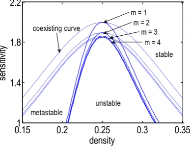
 in the space (;a) respectively. The neutral stability curves and the coexisting curves are shown in Figure 1 for different number m on single lane. Where h_c4, 0.1 and 0.3.

The apex of each line represents the critical point (_c;a_c). The solid lines represent the neutral stability lines and the dashed lines show the coexisting curves for m1,2,3 and 4, respectively. It can be seen in Figure 1 that the space is divided into three regions including the stable region, the metastable region and the unstable region. The sensitivity of critical points, the neutral stability curves and the coexisting curves decrease gradually with the increase of the number m. Moreover, the unstable region shrinks with more optimal current differences’ anticipation effect. It implies that the traffic flow can be further stabilized with the consideration of the information of more front sites of optimal current differences’ anticipation effect. As m=3,4, corresponding curves are almost coincided. It is a conclusion that the effect of only three front sites (m=3) is enough to guarantee the traffic stable under small disturbance. Then m=3 is said as the optimal state for our lattice model.

1.4 1.8 2.2 se nsit ivit y

m = 1 m = 2

m = 3 m = 4 coexisting curve

unstable

[image:4.595.64.534.97.570.2] [image:4.595.197.392.618.767.2]

Numerical Simulation

In this section, the initial conditions are assumed as follows:

    

 

 

 

 

 



51 :

) 0 ( ) 1 (

50 :

) 0 ( ) 1 (

51 , 50 :

) 0 ( ) 1 (

0 0 0

j j j

j j

j j

j j

  



  



 



(20)

where the initial disturbance 0.1,a1/ 1.89,_c ₀0.25, 0.1,0.3and the total number of sitesN100. And the periodic boundary condition is adopted for numerical simulation.

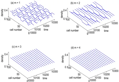
Figure 2 shows the simulation results after 4

10 time steps under the different numberm. From

Figure 2, it can be seen that the kink–antikink soliton solutions propagate backwards. From pattern (a) to pattern (d) in Figure 2, it is obvious that the traffic jams abate gradually with the increase of m. According to figs. 2(a) and (b), the traffic flow is unstable because the unstable condition (12) is satisfied as m=1,2 with a small disturbance inserted into the uniform traffic flow, which results in appearing the propagating backward kink–antikink density wave.

0

10100 10200

10300

0 50 100

0.1 0.4

time 10000

cell number (a) m = 1

de

nsit

y

0 10100

10200 10300

0 50 100 0.1 0.4

time 10000

(b) m = 2

cell number

de

nsit

y

10100 10200

10300

0 50 100 0.1 0.4

time 10000

(c) m = 3

cell number

de

nsit

y

10100 10200

10300

0 50 100 0.1 0.4

time 10000

(d) m = 4

cell number

de

nsit

[image:5.595.86.503.300.589.2]

y

Figure 2. Spatiotemporal evolutions of density when  0.3 and 0.1 _fora1.89.

0 20 40 60 80 100 0.2

0.22 0.24 0.26 0.28

cell number

de

nsit

y

(a) m=1

0 20 40 60 80 100

0.2 0.22 0.24 0.26 0.28

cell number

de

nsit

y

(b) m = 2

0 20 40 60 80 100

0.2 0.22 0.24 0.26 0.28

cell number

de

nsit

y

(c) m = 3

0 20 40 60 80 100

0.2 0.22 0.24 0.26 0.28

cell number

de

nsit

y

[image:6.595.88.498.72.395.2]

(d) m = 4

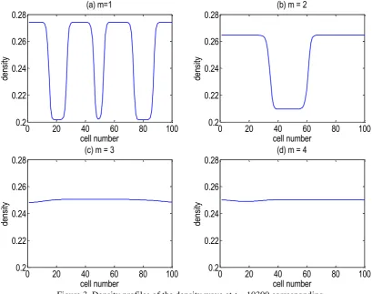
Figure 3. Density profiles of the density wave at t = 10300 corresponding to the panels in Figure 2 respectively.

Conclusion

In this paper, we propose a new lattice model of traffic flow by considering multiple optimal current differences’ anticipation effect on single lane. Linear analyses are carried out to get the stability criterion. Nonlinear analyses are performed to derive the mKdV equation near the critical point and obtain kink–antikink soliton solution to describe the traffic flow density. It is concluded that multiple optimal current differences’ anticipation effect did improve the stability of traffic flow significantly. Moreover, we find that the m=3 is the optimal anticipation states. The simulation results are in good accordance with the theoretical analyses. Therefore, it is reasonable to conclude that multiple optimal current differences’ anticipation effect should be considered in lattice models.

Acknowledgments

This work was supported by the National Natural Science Foundation of China (61673168), the Scientific Research Fund of Hunan Provincial Education Department, China (Grant No. 15A132, No.14C0793), the Second Phase of Doctor Scientific Research Startup Project Foundation of Hunan University of Arts and Science, China (Grant No. 14BSQD13) and the Scientific Research Project Foundation of Hunan University of Arts and Science, China (Grant No. 16ZD05).

References

[5] H.X. Ge, Physica A 388 (2009) 1682.

[6] H.X. Ge, R.J. Cheng, L. Lei, Physica A 389 (2010) 2825.

[7] Z.P. Li, X.L. Li, F.Q. Liu, Int. J. Mod. Phys. C 19 (2008) 1163.

[8] Z.P. Li, F.Q. Liu, J. Sun, China Phys B 20 (2011) 088901.

[9] Z.P. Li, R. Zhang, S.Z. Xu, Y.Q. Qian, Commun Nonlinear Sci Numer Simulat 24 (2015) 52.

[10] T. Nagatani, Physica A 271 (1999) 200.

[11] T. Nagatani, Phys. Rev. E 59 (1999) 4857.

[12] T. Nagatani, Physica A 272 (1999) 592.

[13]W.X. Zhu, Commun. Theor. Phys. 50 (2008) 753.

[14]W.X. Zhu, E.X. Chi, Int. J. Mod. Phys. C. 19 (2008) 727.

[15] D. H. Sun, M. Zhang, T. Chuan, Modern Physics Letters B 28 (2014) 1450091.

[16] C. Tian, D.H. Sun, M. Zhang, Commun Nonlinear Sci Numer Simulat 16 (2011) 4524.

[17]T. Nagatani, Physica A 265 (1999) 297.

[18]T.Q. Tang, H.J. Huang, Y. Xue, Acta Phys. Sin. 55 (2006) 4026.

[19] T.Q. Tang, C.Y. Li, H.J. Huang, Phys. Lett. A 374 (2010) 3951.

[20] T.Q. Tang, H.J. Huang, H.Y. Shang, Phys. Lett. A 374 (2010) 1668.

[21] G.H. Peng, R.J. Cheng, Physica A 392 (2013) 3563.

[22] G.H. Peng, W. Song, Y.J. Peng, S.H. Wang, Physica A 398 (2014) 76.

[23] G.H. Peng, X.H. Cai, C.Q. Liu, B.F. Cao, Physics Letters A 375 (2011) 2153.

[24] G.H. Peng, Commun Nonlinear Sci Numer Simulat 18 (2013) 2801.

[25] A.K. Gupta, P. Redhu, Physica A 392 (2013) 5622.

[26] A.K. Gupta and P. Redhu, Nonlinear Dynam. 76 (2014) 1001.

[27] G.H. Peng, Modern Physics Letters B, 29, (2015) 1550174.