Application of Conjugate Gradient Approach for Nonlinear Optimal Control Problem with Model Reality Differences

(1)

ISSN Online: 2152-7393 ISSN Print: 2152-7385

DOI: 10.4236/am.2018.98064 Aug. 29, 2018 940 Applied Mathematics

Application of Conjugate Gradient Approach

for Nonlinear Optimal Control Problem with

Model-Reality Differences

Sie Long Kek

1

_{, Wah June Leong}

2

_{, Sy Yi Sim}

3

_{, Kok Lay Teo}

4

1_{Department of Mathematics and Statistics, Universiti Tun Hussein Onn Malaysia, Campus Pagoh, Panchor, Malaysia} 2_{Department of Mathematics, Universiti Putra Malaysia, Serdang, Malaysia}

3_{Department of Electrical Engineering Technology, Universiti Tun Hussein Onn Malaysia, Campus Pagoh, Panchor, Malaysia} 4_{Department of Mathematics and Statistics, Curtin University of Technology, Perth, Australia}

Abstract

In this paper, an efficient computational algorithm is proposed to solve the nonlinear optimal control problem. In our approach, the linear quadratic op-timal control model, which is adding the adjusted parameters into the model used, is employed. The aim of applying this model is to take into account the differences between the real plant and the model used during the calculation procedure. In doing so, an expanded optimal control problem is introduced such that system optimization and parameter estimation are mutually inter-active. Accordingly, the optimality conditions are derived after the Hamilto-nian function is defined. Specifically, the modified model-based optimal con-trol problem is resulted. Here, the conjugate gradient approach is used to solve the modified model-based optimal control problem, where the optimal solution of the model used is calculated repeatedly, in turn, to update the ad-justed parameters on each iteration step. When the convergence is achieved, the iterative solution approaches to the correct solution of the original optim-al control problem, in spite of model-reoptim-ality differences. For illustration, an economic growth problem is solved by using the algorithm proposed. The results obtained demonstrate the efficiency of the algorithm proposed. In conclusion, the applicability of the algorithm proposed is highly recom-mended.

Keywords

Nonlinear Optimal Control, Conjugate Gradient Approach, Iterative Solution, Adjusted Parameters, Model-Reality Differences

How to cite this paper: Kek, S.L., Leong, W.J., Sim, S.Y. and Teo, K.L. (2018) Appli-cation of Conjugate Gradient Approach for Nonlinear Optimal Control Problem with Model-Reality Differences. Applied Ma-thematics, 9, 940-953.

https://doi.org/10.4236/am.2018.98064

Received: July 12, 2018 Accepted: August 26, 2018 Published: August 29, 2018

http://creativecommons.org/licenses/by/4.0/

(2)

DOI: 10.4236/am.2018.98064 941 Applied Mathematics

1. Introduction

Recently, the integrated optimal control and parameter estimation (IOCPE) al-gorithm has been proposed [1] in solving the nonlinear optimal control problem, both for discrete time deterministic and stochastic cases (see for more detail in

[2]-[9]). In essence, the concept of the IOCPE algorithm is come from the

dy-namic integrated system optimization and parameter estimation (DISOPE) al-gorithm, which was developed by [10]. By using the DISOPE algorithm, optimal control of the deterministic dynamical systems, not only for continuous time but also for discrete time, has been widely discussed [10][11]. On this point of view, the applications of the DISOPE algorithm have been well-defined. Date back to the 70s, [12] and [13] proposed the integrated system optimization and parame-ter estimation (ISOPE) algorithm, which is for solving the static optimization problems. Since then, the development of ISOPE algorithm in the dynamic ver-sion is rapidly growing up till today.

In fact, the basic idea for ISOPE, DISOPE and IOCPE algorithms is the prin-ciple of model-reality differences [1][10][13]. Because the structure of the non-linear optimal control problem is complex and solving such problem is compu-tationally demanding, the simplified model for the original optimal control problem is proposed to be solved iteratively. By adding the adjusted parameters into the model used, the differences between the model used and the real plant can be measured. This measurement is done repeatedly, in turn, to update the optimal solution of the model used. Once the convergence is achieved, the itera-tive solution approximates to the true optimal solution of the original optimal control problem, in spite of model-reality differences [1] [10][13]. Besides, for solving the discrete time nonlinear stochastic optimal control problem, the Kal-man filtering theory is associated with the principle of model-reality differences in order to do state estimation and system optimization [2][3][4][6].

By virtue of the evolution of these algorithms, the feedback optimal control law is provided in solving the nonlinear optimal control problems, and their ef-fectiveness has been well-confirmed. Nevertheless, the applicability of the open-loop optimal control law in these algorithms shall be investigated such that the popularity of these algorithms could be promoted. This is because of the open-loop optimal control sequences could be generated by taking the advantage of the power of the state-of-the-art nonlinear programming (NLP) solver. Thus, as an efficient optimization technique, the conjugate gradient method [14][15]

has been explored to solve the optimal control problem [16][17][18] since last few decades. Thereby, the use of the conjugate gradient method inspires us to explore this method in the IOCPE algorithm practically.

(3)

DOI: 10.4236/am.2018.98064 942 Applied Mathematics for optimality is derived. Consequently, the modified model-based optimal con-trol problem is converted to be a nonlinear optimization problem. By applying the conjugate gradient approach, the nonlinear optimization problem is solved and the optimal control sequences are generated. With this open-loop control law, the dynamical system is optimized and the cost function is evaluated. For illustration, optimal control of an economic growth problem [19] is discussed. The results obtained show the applicability of the algorithm proposed.

The structure of the paper is organized as follows. In Section 2, the problem statement is described briefly, where the simplified model from the nonlinear optimal control problem is discussed. In Section 3, system optimization with parameter estimation is further discussed. The use of the conjugate gradient ap-proach in solving the model-based optimal control problem is presented and the calculation procedure is summarized as an iterative algorithm. In Section 4, an economic growth problem is solved and the results are obtained. Finally, the concluding remarks are made.

2. Problem Statement

Consider a general discrete-time optimal control problem, given by

( )

(

( )

)

(

( ) ( )

)

(

)

(

( ) ( )

)

( )

1 0

0

min , , ,

subject to 1 , , , 0

N

u k J u x N N _k L x k u k k

x k f x k u k k x x

ϕ −

=

= +

+ = =

∑

₍₁₎

where _{u k}

( )

_∈ℜm,_k₌0,1, ,_ _N₋1_and _{x k}

( )

_∈ℜn_,_k₌_{0,1, ,}_ _N_{are, respectively,}

the control sequences and the state sequences. Here, _f :_{ℜ × ℜ × ℜ → ℜ}n m n

represents the real plant, _L:_{ℜ × ℜ × ℜ → ℜ}n m _{is the cost under summation}

and _{ϕ ℜ ×ℜ → ℜ}: n _{is the terminal cost, whereas}

0

J is the scalar cost func-tion and x0 is the known initial state vector. It is assumed that all functions in Equation (1) are continuously differentiable with respect to their respective ar-guments.

This problem is regarded as the real optimal control problem, and is referred to as Problem (P). Note that the structure of Problem (P) is complex and nonli-near, solving Problem (P) requires the efficient computation techniques. On this point of view, the simplified model of Problem (P) is probably suggested to be solved in order to approximate the true optimal solution of Problem (P). There-fore, let us define this simplified model-based optimal control problem as fol-lows:

( )

( ) ( ) ( ) ( )

( )

( ) ( )

( )

(

)

( )

(

)

( )

( ) ( )

T 1

1 _T _T

0

1 min

2 1 2

subject to 1 , 0

u k

N

k

J u x N S N x N N

x k Qx k u k Ru k k

x k Ax k Bu k k x x

γ

γ α

−

=

= +

+ + +

+ = + + =

∑

(2)

where γ

( )

k k, =0,1, ,_ N_andα

( )

k k, =0,1, ,_ N−1_{are introduced as the} ad-justed parameters, whereas A is an n n× _{transition matrix and}_B_{is an}n m×

(4)

DOI: 10.4236/am.2018.98064 943 Applied Mathematics matrices, and R is a m m× _{positive definite matrix. Here,} J₁ is the scalar cost function.

This problem is referred to as Problem (M).

Notice that, due to the different structures and parameters, only solving Prob-lem (M), without the adjusted parameters, would not obtain the optimal solu-tion of Problem (P). However, by adding the adjusted parameters into Problem (M), the differences between the real plant and the model used can be calculated. In such a way, solving Problem (M) iteratively could give the correct optimal solution of Problem (P), in spite of model-reality differences.

3. System Optimization with Parameter Estimation

Now, introduce an expanded optimal control problem, which is referred to as Problem (E), given by

( )

( ) ( ) ( ) ( )

(

( )

( ) ( )

( )

)

( )

( ) ( )

(

)

( )

( ) ( )

( ) ( ) ( ) ( )

(

( )

)

1

T T T

2

0

2 2

1 2

0

T

1 1

min

2 2

1 1

2 2

subject to 1 , 0

1 _,

2

N

u k J u x N S N x N N _k x k Qx k u k Ru k

k r u k v k r x k z k

x k Ax k Bu k k x x

z N S N z N N z N N

γ

α

γ ϕ

−

=

= + + +

+ + − + −

+ = + + =

+ =

∑

( )

( ) ( )

( )

(

)

( )

(

( ) ( )

)

( )

(

( ) ( )

)

( )

T T

1 _, _,

2

, ,

z k Qz k v k Rv k k L z k v k k

Az k Bv k k f z k v k k

v k u k z k x k

γ α

+ + =

= =

(3)

where _{v k}

( )

_∈ℜm,_k₌0,1, ,_ _N₋1_and _{z k}

( )

_∈ℜn_,_k₌_{0,1, ,}_ _N _are

intro-duced to separate the sequences of control and state in the optimization problem from the respective signals in the parameter estimation problem, and ⋅ _de

notes the usual Euclidean norm. The term 1₂r u k1

( ) ( )

−v k 2 and

( ) ( )

2 2

1

2r x k −z k with r r1 2, ∈ℜ are introduced to improve the convexity and to facilitate the convergence of the resulting iterative algorithm. Here, it is classi-fied that the algorithm is designed such that the constraints v k

( ) ( )

=u k _and

( ) ( )

z k =x k _{are satisfied upon termination of the iterations, assuming that} convergence is achieved. Moreover, the state constraint z k

( )

and the control constraint v k

( )

are used for the computation of the parameter estimation and matching scheme, while the corresponding state constraint x k

( )

and control constraint u k

( )

are reserved for optimizing the model-based optimal control problem. By virtue of this, system optimization and parameter estimation are mutually integrated.

(5)

( )

(

( )

( ) ( )

( )

)

( )

( ) ( )

(

)

(

( )

)

( ) ( )

T T 2 2 2 1 2 T T T 1 2 1 1 2 2 1

H k x k Qx k u k Ru k k

r u k v k r x k z k

p k Ax k Bu k k

k u k k x k

γ α λ β = + + + − + − + + + + − − (4)

where _λ

( )

_k _∈ℜm,_k₌0,1, ,_ _N₋1_, _β

( )

_k _∈ℜn_,_k₌_{0,1, ,}_ _N_and

( )

n, 0,1, ,

p k ∈ℜ k=  N are modifiers. Then, the augmented cost function be-comes

( )

( ) ( ) ( ) ( )

( ) ( )

( )

(

( )

)

( ) ( ) ( ) ( )

( ) ( )

(

)

( ) ( )

( )

(

( ) ( )

)

(

( )

( ) ( )

( )

)

( )

(

( ) ( )

)

( )

)

T T T

2

T

1 _T _T _T

T

2 0

T T

T

1 ₀ ₀

2 1 , 2 ( ) 1 , , 2 , , N k

J u x N S N x N N p x p N x N

N z N N z N S N z N N

x N z N H k p k x k k v k k z k

k L z k v k k z k Qz k v k Rv k k

k f z k v k k Az k Bv k k

γ

ξ ϕ γ

λ β ξ γ µ α − = ′ = + + −   + _ − − _  

+ Γ − + − + +

  + _ − + − _   + − − −

∑

(5) where p k

( ) ( ) ( ) ( ) ( )

,ξ k ,λ k ,β k ,µ k _and Γ are the appropriate multipliers to be determined later.

Applying the calculus of variation [20][21][22], the following necessary con-ditions for optimality are obtained:

1) Stationary condition:

( )

T

(

)

( )

(

( ) ( )

)

1

1 0

Ru k +B p k+ −λ k +r u k −v k = (6a) 2) Co-state equation:

( )

T

(

)

( )

(

( ) ( )

)

2

1

p k =Qx k +A p k+ −β k +r x k −z k _(6b) 3) State equation:

(

1

)

( )

x k+ =Ax k +Bu k +α k _(6c) 4) Boundary conditions:

( )

( ) ( )

p N =S N x N + Γ_and x

( )

0 =x₀_(6d)

5) Adjusted parameter equations:

( )

(

)

1

( ) ( ) ( ) ( )

T ,

2

z N N z N S N z N N

ϕ = +γ _(7a)

( ) ( )

(

)

1

(

( )

T

( ) ( )

T

( )

)

( )

, ,

2

L z k v k k = z k Qz k +v k Rv k +γ k _(7b)

( ) ( )

(

, ,

)

( )

f z k v k k =Az k +Bv k +α k (7c) 6) Modifier equations:

( )

( ) ( )

z Nϕ S N z N

(6)

( )

(

( )

)

_{( )}

(

)

T

ˆ 1

v k

f

k L Rv k B p k

v k

λ = − ∇ − −_ ∂ − _ + ∂

  (8b)

( )

(

( )

)

_{( )}

(

)

T

ˆ 1

z k f

k L Qz k A p k

z k

β = − ∇ − −_ ∂ − _ + ∂

  (8c)

with ξ

( )

k =1_and µ

( )

k =p kˆ

(

+1

)

_. 7) Separable variables:

( ) ( )

v k =u k _, z k

( ) ( )

=x k _, p kˆ

( )

=p k

( )

_{. (9)} Notice that the parameter estimation problem is defined by Equation (7) and the computation of multipliers is given by Equation (8). Indeed, the necessary conditions, which are defined by Equations (6a) to (6d), are the optimality for the modified model-based optimal control problem.

3.2. Modified Model-Based Optimal Control Problem

The modified model-based optimal control problem, which is referred to as Problem (MM), is given by

( )

( ) ( ) ( )

( ) ( )

( )

( ) ( )

( )

(

)

( )

( ) ( )

(

)

( )

( ) ( )

T T

3

1 _T _T

0

2 2

1 2

T T

0 1

min

2 1 2

1 1

2 2

subject to 1 , 0

u k

N

k

J u x N S N x N x N N

x k Qx k u k Ru k k

r u k v k r x k z k

k u k k x k

x k Ax k Bu k k x x

γ

λ β

α

−

=

= + Γ +

+ + +

+ − + −

− −

+ = + + =

∑

(10)

with the specified α

( ) ( ) ( ) ( )

k ,γ k ,λ k ,β k , ,Γ v k

( )

_and z k

( )

, where the boundary conditions are given by x0 and p N

( )

with the specified multiplier

Γ.

3.3. Open-Loop Optimal Control Law

For simplicity, define Problem (MM) as an equivalent nonlinear optimization problem with the initial control _u( )0 ₌_{u k}

( )

0_{, given by}

( ) 3

( )

min

u k J u subject to

m

u∈ℜ _for k=0,1, , N−1 (11)

where the admissible control variable u is set to be

( )

(

)

T

(

( )

)

T

(

)

T

0 , 1 , , 1

u=__u u  u N− __.

(7)

( )

3 u k

J u H

∇ = ∇ ₍₁₂₎

which can be calculated from the Hamiltonian function (4) and the stationary condition (6a) once the necessary conditions for optimality, given by Equations (6) - (9), are satisfied.

Suppose the gradient function (12) is represented as

( )

u k( )

g u = ∇ H. (13)

Then, for arbitrary initial control _u( )0 _{, the initial gradient and the initial} di-rection are, respectively, given by

( )0

( )

( )0

g =g u and _d( )0 _{= −}_g( )0 _{. (14)}

By using the line search equation [14][16], the control sequences can be gen-erated from

( )i1 ( )i ( )i i

u + ₌u _{+ ⋅}a d ₍₁₅₎ where ai∈ℜ is determined from the one-dimensional search, that is,

( ) ( )

(

)

3 0

arg min i i i

a

a J u a d

≥

= + ⋅ . (16)

Later, the gradient and the direction are updated as follow: ( )i1

( )

( )i1

g + ₌g u + ₍₁₇₎

( )i1 ( )i1 ( )i i

d + _{= −}g + _{+ ⋅}b d

(18) with the coefficient

( ) ( ) ( ) ( )

1 T 1

T

i i

i i i

g g

b

g g

+ +

= ₍₁₉₎

where i=0,1,2,__{represents the iteration numbers.}

Thus, we present the result on the obtaining optimal control law discussed above as a proposition, given below:

Proposition 1. Consider Problem (N). The control sequences _u( )i _,_{which is}

defined in Equation (15) and is represented by

( )

₍

_{( )}

₎

T

₍

_{( )}

₎

T

₍

₎

T

0 , 1 , , 1

i

u =_u u u N− _

  ,

is generated through a set of the direction vectors _d( )i _{whose components are}

linearly independent. Also, the direction _d( )i _{is conjugacy}_. Proof: Refer [14].

Here, the conjugate gradient algorithm for obtaining the optimal control law is summarized below:

Algorithm 1: Conjugate gradient algorithm

Data Choose the arbitrary initial control _u( )0 _{. Compute the initial gradient} ( )0

g and the initial direction _d( )0 _{from Equation (14). Set} _i_{= 0.}

(8)

DOI: 10.4236/am.2018.98064 947 Applied Mathematics Step 2 Solve the costate Equation (6b) backward in time from k = N to k = 0 with the boundary condition (6d), where p k

( )

i is the solution obtained.

Step 3 Calculate the value of the cost functional J u3

( )

( )i from Equation (10). Step 4 Determine the step size ai from Equation (16).

Step 5 Update the control _u( )i+1 _{from Equation (15).}

Step 6 Update the gradient _g( )i+1 _{from Equation (17). If the gradient} ( )i1 ₀

g + ₌ _{, stop, else go to Step 7.}

Step 7 Compute the coefficient bi from Equation (19).

Step 8 Update the direction _d( )i+1 _{from Equation (18). Set}_{i i}_{= +}₁_{, go to} Step 1.

Remarks:

1) The initial control _u( )0 _{can be any valued-vectors, including the zero} vec-tor.

2) The gradient function g u

( )

for Problem (N) defined by Equation (11) is calculated from the stationary condition (6a). This is the turning point of using the conjugate gradient algorithm for solving Problem (M) defined by Equation (2) and Problem (MM) defined by Equation (10).

3) The optimal control sequences generated by the line search equation in Equation (15) is known as the open-loop control law.

4) The necessary conditions (6b) and (6c) shall be satisfied in solving Problem (N) defined by Equation (11).

3.4. Iterative Procedure

Accordingly, from the discussion above, a summary of the calculation procedure for the integrated system optimization and parameter estimation is made as fol-lows:

Algorithm 2: Iterative procedure

Data A B Q R S N N x r r k k k f L, , , ,

( )

, , , , , , , , ,0 1 2 v z p . Note that A and B could be

determined based on the linearization of f at x0 or from the linear terms of f . Step 0 Compute a nominal solution. Assume that α

( )

k =0,k=0,1, ,_ N−1 and r r1= =2 0 . Solve Problem (M) defined by Equation (2) to obtain

( )

0_, _{0,1, ,} ₁

u k k=  N− and _{x k}

( )

0_,_{p k}

( )

0_,_k₌_{0,1, ,}_N

 . Then, with

( )

k 0,k 0,1, ,N 1

α = =  − and using r r1 2, from the data. Set i=0 ,

( )

0

( )

0

v k =u k , _{z k}

( )

0₌_{x k}

( )

0_and _{p k}_ˆ

_{( )}

0 ₌_{p k}

_{( )}

0_.

Step 1 Compute the parameters γ

( )

k ki, =0,1, ,_ N_and

( )

k ki, 0,1, ,N 1

α =  − from Equation (7). This is called the parameter estima-tion step.

Step 2 Compute the modifiers _Γi,_λ

( )

_k i_and _β

( )

_{k k}i_, ₌_{0,1, ,}_N₋₁

 from

Equation (8). Notice that this step requires taking the derivatives of f and L with respect to _{v k}

( )

i_and _{z k}

_{( )}

i_.

Step 3 With _γ

( ) ( )

_k i,_α _k i, ,_Γi _λ

( ) ( ) ( )

_k i,_β _{k v k}i, i_and

_{( )}

i

z k , solve Problem (N) by using Algorithm 1. This is called the system optimization step.

(9)

DOI: 10.4236/am.2018.98064 948 Applied Mathematics b) Use Equation (6c) to obtain the new state x k k

( )

i, =0,1, ,_ N_.

c) Use Equation (6b) to obtain the new costate p k k

( )

i, =0,1, ,_ N_.

Step 4 Test the convergence and update the optimal solution of Problem (P). In order to provide a mechanism for regulating convergence, a simple relaxation method is employed:

( )

i1

( )

i

(

( )

i

( )

i

)

v

v k + v k k u k v k

= + − _(20a)

( )

i1

( )

i

(

( )

i

( )

i

)

z

z k + z k k x k z k

= + − _(20b)

( )

1

( )

(

( )

)

ˆ i ˆ i i ˆ i

p

p k + = p k +k p k −p k _(20c)

where k k kv, ,z p∈

(

0,1

]

are scalar gains. If

( )

1

( )

, 0,1, , 1 i i

v k + ₌v k k₌ N₋



and z k

( )

i+1=z k k

( )

i, =0,1, ,_ N _{, within a given tolerance, stop; else set}

1

i i= + , and repeat the procedure starting from Step 1. Remarks:

1) The variable α

( )

k _{is zero in Step 0. The calculated value of}α

( )

k _changes from iteration to iteration during the calculation procedure.

2) The conjugate gradient algorithm is applied to generate the control se-quences u k

( )

for Problem (M) and Problem (MM), respectively.

3) Problem (P) is not necessary to be linear or to have a quadratic cost func-tion.

4) The conditions

( )

i 1

( )

i u k + ₌u k

and

( )

i1

( )

i x k + ₌x k

are required to be sa-tisfied for the converged optimal control sequence and the converged state se-quence. The following averaged 2-norms are computed and then they are com-pared with a given tolerance to verify the convergence of u k

( )

and x k

( )

:

( )

1 2

1 ₁

1

2 ₀

1 1

N _i _i

i i

k

u u u k u k

N − ₊ + =   − =_ − _ −



∑

 (21a)

( )

1

( )

1 2

1

2 ₀

1 N _i _i

i i

k

x x x k x k

N + + =   − =_ − _



∑

 (21b)

5) The convergence result on the conjugate gradient algorithm can be referred to [14], and the convergence result for Algorithm 2 is presented in [4] and [10].

4. Illustrative Example

Consider a basic economic growth model [19][23], which is a discrete time mi-nimization problem, given by

( )

(

( ) ( )

)

(

)

(

( ) ( )

)

( )

1 0

0

min , ,

subject to 1 , , , 0 5

N k

u k J u _k L x k u k k

x k f x k u k k x

ρ − = = + = =

∑

where the payoff function and dynamics system are, respectively, defined by

( ) ( )

(

, ,

)

ln

(

( )

)

(10)

fac-DOI: 10.4236/am.2018.98064 949 Applied Mathematics tor, whereas _Λxν_{is a production function with constants}_{Λ >}₀_, ₀_{< <}_ν ₁_.

The difference between the output and the next period’s capital stock is the consumption.

Let us refer this problem as Problem (P). In literature, the exact solution of Problem (P) is known [24], and is given by

( )

ln

( )

,

V x = +C D x

with

(

)

(

)

(

)

ln 1 ln

1 D

C= − ⋅ν ρ ⋅ Λ + ⋅ ⋅_ρ ρ ν ρ⋅ ⋅ Λ

− and D 1

ν ν ρ =

− ⋅ .

The unique optimal equilibrium for Problem (P) is given by

( ) *

1

x _ν

ν ρ

−

=

⋅ ⋅ Λ.

By using the specified parameters Λ =5, ν =0.34 and ρ =0.95_{, the} op-timal equilibrium is _x*_≈_2.0673 _[23]_.

In the following, we introduce a simplified model-based optimal control mod-el, which is derived from Problem (P) and is referred to as Problem (M), given below:

( )

(

( )

)

( )

(

) ( ) ( )

( ) ( )

30 ₂ ₂

1

0 1

min 0.1 10

2

subject to 1 , 0 5.

u k J u _k x k u k k

x k x k u k k x

γ α

=

 

= _ ⋅ + ⋅ + _

 

+ = + + =

∑

Note that Problem (M) and Problem (P) are different from the structures and the parameters used.

After running the algorithm proposed within the tolerance (10−6_{), the result is}

shown in Table 1. The initial cost, which is 13.072, is the cost spent before tak-ing into account system optimization with parameter estimation. At the end of implementing the algorithm proposed, the final cost is 22.198. There are 41 ite-rations with 7.84 seconds to reach the convergence.

The graphical results for this economic growth model illustrate the applica-tion of the algorithm proposed. Figure 1 shows the final control trajectory and

Figure 2 shows the final state trajectory, respectively. With this final control

so-lution, it is observed that the final state towards to the steady state at x = 2.0673.

Figure 3 shows the final costate trajectory, while Figure 4 and Figure 5 show,

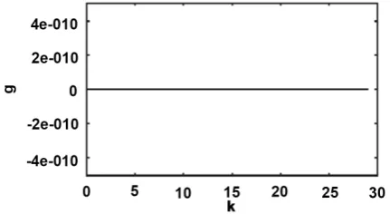
respectively, the adjusted parameters γ(k) and α(k). Overall, these solutions are in the optimal sense, which are verified by the satisfaction of the stationary con-dition shown in Figure 6.

5. Concluding Remarks

(11)

Table 1. Simulation result.

Iteration Number Initial Cost Final Cost Elapsed Time (s)

[image:11.595.202.547.96.644.2]

41 13.072 22.198 7.84008

Figure 1. Final control trajectory u k

( )

.

[image:11.595.267.481.335.499.2]

Figure 2. Final state trajectory x k

( )

(--) and state equili-brium _x*₍_{⋅⋅⋅⋅⋅}_).

[image:11.595.271.480.539.704.2]

(12)

[image:12.595.272.477.75.240.2]

[image:12.595.267.478.279.448.2]

Figure 4. Adjusted parameter γ

( )

k .

[image:12.595.266.482.482.600.2]

Figure 5. Adjusted parameter α

( )

k .

Figure 6. Stationary condition g.

(13)

re-DOI: 10.4236/am.2018.98064 952 Applied Mathematics peatedly, are taken into consideration during the iteration calculation procedure. At the convergence, the optimal solution of the model used approximates to the true optimal solution of the original optimal control problem, in spite of mod-el-reality differences. For illustration, the application of the algorithm proposed was discussed for solving a basic economic growth model. The results obtained show the efficiency of the algorithm proposed. In conclusion, the applicability of the algorithm is highly recommended.

Acknowledgements

The authors would like to acknowledge the Universiti Tun Hussein Onn Malay-sia (UTHM) and the Ministry of Higher Education (MOHE) for the financial support for this study under the research grant FRGS VOT. 1561.

Conflicts of Interest

The authors declare no conflicts of interest regarding the publication of this pa-per.

References

[1] Kek, S.L., Teo, K.L. and Mohd Ismail, A.A. (2010) An Integrated Optimal Control Algorithm for Discrete-Time Nonlinear Stochastic System. International Journal of Control, 83, 2536-2545. https://doi.org/10.1080/00207179.2010.531766

[2] Kek, S.L., Teo, K.L. and Mohd Ismail, A.A. (2012) Filtering Solution of Nonlinear Stochastic Optimal Control Problem in Discrete-Time with Model-Reality Differ-ences. Numerical Algebra, Control and Optimization, 2, 207-222.

https://doi.org/10.3934/naco.2012.2.207

[3] Kek, S.L., Mohd Ismail, A.A., Teo, K.L. and Rohanin, A. (2013) An Iterative Algo-rithm Based on Model-Reality Differences for Discrete-Time Nonlinear Stochastic Optimal Control Problems. Numerical Algebra, Control and Optimization, 3, 109-125. https://doi.org/10.3934/naco.2013.3.109

[4] Kek, S.L., Teo, K.L. and Mohd Ismail, A.A. (2015) Efficient Output Solution for Nonlinear Stochastic Optimal Control Problem with Model-Reality Differences. Mathematical Problems in Engineering, 2015, Article ID: 659506.

https://doi.org/10.1155/2015/659506

[5] Kek, S.L., Mohd Ismail, A.A. and Teo, K.L. (2015) A Gradient Algorithm for Op-timal Control Problems with Model-Reality Differences. Numerical Algebra, Con-trol and Optimization, 5, 252-266.

[6] Kek, S.L. and Mohd Ismail, A.A. (2015) Output Regulation for Discrete-Time Non-linear Stochastic Optimal Control Problems with Model-Reality Differences. Nu-merical Algebra, Control and Optimization, 5, 275-288.

https://doi.org/10.3934/naco.2015.5.275

[7] Kek, S.L., Li, J. and Teo, K.L. (2017) Least Squares Solution for Discrete Time Non-linear Stochastic Optimal Control Problem with Model-Reality Differences. Applied Mathematics, 8, 1-14. https://doi.org/10.4236/am.2017.81001

(14)

DOI: 10.4236/am.2018.98064 953 Applied Mathematics [9] Kek, S.L., Sim, S.Y., Leong, W.J. and Teo, K.L. (2018) Discrete-Time Nonlinear

Stochastic Optimal Control Problem Based on Stochastic Approximation Approach. Advances in Pure Mathematics, 8, 232-244. https://doi.org/10.4236/apm.2018.83012 [10] Becerra, V.M. and Roberts, P.D. (1996) Dynamic Integrated System Optimization

and Parameter Estimation for Discrete Time Optimal Control of Nonlinear Sys-tems. International Journal of Control, 63, 257-281.

https://doi.org/10.1080/00207179608921843

[11] Roberts, P.D. and Becerra, V.M. (2001) Optimal Control of a Class of Discrete-Continuous Nonlinear Systems Decomposition and Hierarchical Structure. Automatica, 37, 1757-1769. https://doi.org/10.1016/S0005-1098(01)00141-8

[12] Roberts, P.D. (1979) An Algorithm for Steady-State System Optimization and Pa-rameter Estimation. International Journal of Systems Science, 10, 719-734. https://doi.org/10.1080/00207727908941614

[13] Roberts, P.D. and Williams, T.W.C. (1981) On an Algorithm for Combined System Optimization and Parameter Estimation. Automatica, 17, 199-209.

https://doi.org/10.1016/0005-1098(81)90095-9

[14] Chong, E.K.P. and Zak, S.H. (2013) An Introduction to Optimization. 4th Edition, John Wiley & Sons, Inc., Hoboken, New Jersey.

[15] Mostafa, E.M.E. (2014) A Nonlinear Conjugate Gradient Method for A Special Class of Matrix Optimization Problems. Journal of Industrial and Management Op-timization, 10, 883-903. https://doi.org/10.3934/jimo.2014.10.883

[16] Lasdon, L.S. and Mitter, S.K. (1967) The Conjugate Gradient Method for Optimal Control Problems. IEEE Transactions on Automatic Control, 12,132-138.

https://doi.org/10.1109/TAC.1967.1098538

[17] Nwaeze, E. (2011) An Extended Conjugate Gradient Method for Optimizing Continuous-Time Optimal Control Problems. Canadian Journal on Computing in Mathematics, Natural Sciences, Engineering & Medicine, 2, 39-44.

[18] Raji, R.A. and Oke, M.O. (2015) Higher-Order Conjugate Gradient Method for Solving Continuous Optimal Control Problems. IOSR Journal of Mathematics, 11, 88-90.

[19] Brock, W.A. and Mirman, L. (1972) Optimal Economic Growth and Uncertainty: The Discounted Case. Journal of Economy Theory, 4, 479-513.

https://doi.org/10.1016/0022-0531(72)90135-4

[20] Bryson, A.E. and Ho, Y.C. (1975) Applied Optimal Control. Hemisphere, Wash-ington DC.

[21] Lewis, F.L., Vrabie, V. and Symos, V.L. (2012) Optimal Control. 3rd Edition, John Wiley & Sons, Inc., New York.https://doi.org/10.1002/9781118122631

[22] Kirk, D.E. (2004) Optimal Control Theory: An Introduction. Dover Publications, New York.

[23] Grüne, L., Semmler, W. and Stieler, M. (2015) Using Nonlinear Model Predictive Control for Dynamic Decision Problems in Economics. Journal of Economic Dy-namics and Control, 60, 112-133.https://doi.org/10.1016/j.jedc.2015.08.010 [24] Santos, M.S. and Vigo-Aguiar, J. (1998) Analysis of a Numerical Dynamic

Pro-gramming Algorithm Applied to Economic Models. Econometrica, 66, 409-426.