Spike train analysis

LEABHARLANN CHOLAISTE NA TRIONOIDE, BAILE ATHA CLIATH TRINITY COLLEGE LIBRARY DUBLIN OUscoil Atha Cliath The University of Dublin

Terms and Conditions of Use of Digitised Theses from Trinity College Library Dublin

Copyright statement

All material supplied by Trinity College Library is protected by copyright (under the Copyright and Related Rights Act, 2000 as amended) and other relevant Intellectual Property Rights. By accessing and using a Digitised Thesis from Trinity College Library you acknowledge that all Intellectual Property Rights in any Works supplied are the sole and exclusive property of the copyright and/or other I PR holder. Specific copyright holders may not be explicitly identified. Use of materials from other sources within a thesis should not be construed as a claim over them.

A non-exclusive, non-transferable licence is hereby granted to those using or reproducing, in whole or in part, the material for valid purposes, providing the copyright owners are acknowledged using the normal conventions. Where specific permission to use material is required, this is identified and such permission must be sought from the copyright holder or agency cited.

Liability statement

By using a Digitised Thesis, I accept that Trinity College Dublin bears no legal responsibility for the accuracy, legality or comprehensiveness of materials contained within the thesis, and that Trinity College Dublin accepts no liability for indirect, consequential, or incidental, damages or losses arising from use of the thesis for whatever reason. Information located in a thesis may be subject to specific use constraints, details of which may not be explicitly described. It is the responsibility of potential and actual users to be aware of such constraints and to abide by them. By making use of material from a digitised thesis, you accept these copyright and disclaimer provisions. Where it is brought to the attention of Trinity College Library that there may be a breach of copyright or other restraint, it is the policy to withdraw or take down access to a thesis while the issue is being resolved.

Access Agreement

By using a Digitised Thesis from Trinity College Library you are bound by the following Terms & Conditions. Please read them carefully.

Spike Train Analysis

Trinity College Dublin

C athal Cooney

A thesis subm itted for the degree of Doctor of Philosophy.

COLLEGS^

2 9 JUL 2015

^ LIBRARY DUBLIN

D eclaration

I dcclarc th a t this tlicsis lias not been sub m itted as an exercise for a

degree at this or any other university and it is entirely niy own work.

I agree to dej)osit this thesis in th e U niversity’s o])en access in stitu ­

tional re])ository or allow the library to do so on niy behalf, subject to

h ish Copyright Legislation and Trinity College Library conditions of use

and acknowledgenieut.

Signed,

C athal Cooney

29th May 2015

A cknow ledgem ents

I w ould like to th a n k niy sui^ervisoi’ C onor H oughton for all his ex p e rtise an d su pi)ort th ro u g h o u t th e eoiuse of niy study. A dditionally, w ith o u t th e sTipport of th e School of M aths, th is thesis would not have b een ])ossit)le.

I w ould also like to th a n k th e Irish R esearch Council for fiuiding m e in these studies.

Sum m ary

This tiiesis focuses on the study of sj^ike trains, the inform ation cariying

signals conveyed by neurons in the nervous system.

Si)iking d a ta from songbirds from [Narayan et al., 2006] was used

l^rominently in this thesis. M ulti-unit d a ta for C hajiter Three was simu­

lated using a model network from [Houghton and Sen, 2008].

In C hapter Two, several clustering algorithm s are introduced. The

eigenvalue algorithm of [Newman, 2006a] to cluster networks wa.s used

j)rominently. This algorithm was combined w ith a measure called the

increm ental m utual inform ation [Singh and Lesica. 2010] to cluster mod­

ules of information in sim ulated networks of neurons.

Chai)ter Three deals mainly w ith two distance measures, th e SPIK E

distance [Kreuz et al., 2013] and the ISI distance [Kreuz et al., 2007].

These distance measures were extended from single-unit to nnilti-unit

measures.

In C hapter Four a simple neuron model is proposed, based on the idea

of sparse coding in the brain. The expected firing rate based on the model

was calculated, and then th e ISI distrib u tio n was calculated from the

firing rate. The calculated distribution was tested against th e empirical

d a ta using the Kolmogorov-Smirnov test for goodness-of-fit [Massey Jr,

1951].

)

C ontents

1 In tr o d u c tio n

1

1.1 Spike t r a i n s ... 2

1.2 Spike tra in m e t r i c s ... 5

1.2.1 V ic to r-P u rp u ra m e t r i c ... C 1.2.2 van Rossum m e t r i c ... 7

1.3 Inform ation T h e o r y ... 9

1.4 D ata sets ... 11

1.4.1 Zel)ra finch d a ta ... 12

1.4.2 M ulti-unit d a t a ... 12

2 C lu ste r in g m e th o d s in sp ik e tra in a n a ly sis

17

2.2 M od ularity ... 19

2.3 N ew m an's eigenvalue a l g o r i t h m ... 22

2.4 New netw ork clustering a l g o r i t h m s ... 27

2.4.1 G enetic a l g o r i th m ... 27

2.4.2 S im ulated ann ealin g ... 29

2.5 A’-m edoids c l u s t e r i n g ... 31

2.6 C lu sterin g res])onses w ith m o d u l a r i t y ... 32

2.7 D is c u s s io n ... 34

3 M a p p in g in fo rm a tio n flow in a sim u la ted n etw o rk o f n eu ­

ron s

37

3.1 T h e bil)liographic i i o t w o r k ... 38

3.2 Iiicreniental m utua! ii if o r n ia t io n ... 39

3.3 X uinerical t e s t i n g ... 40

3.4 D is c u s s io n ... 44

4 M u lti-u n it sp ik e tr a in m e tr ic s

47

4.1.1 ISI d i s t a n c e ... 48

4.1.2 S P IK E d i s t a n c e ... 50

4.2 A ltern ativ e S P IK E d i s t a n c e ... 52

4.3 E xtensions to m u lti-u n it r e c o r d i n g s ... 54

4.3.1 R e s u lt s ... 58

4.4 M iilti-U nit ISI d i s t a n c e ... 60

4.4.1 Single u nit re c o rd in g s ... 60

4.4.2 In itial extension to n u ilti-u n it r e c o r d i n g s ... 61

4.4.3 R e s u lt s ... 63

4.4.4 A ltern ativ e ex tensions to th e m ulti-u n it case . . . 64

4.5 A daj)tive ISI d i s t a n c e s ... 66

4.6 D is c u s s io n ... 69

5 A sim p le n eu ron m o d el

73

5.2 E stim atin g th e firing ra te r { f )... 75

5.3 M arkov P r o c e s s ... 77

5.3.1 E stim atin g th e ra te function r { t ) ... 81

5.3.2 C hange in i)robability w hen a spike arrives . . . . 83

5.3.3 C alcu latin g th e ISI d i s t r i b u t i o n ... 84

5.4 T esting on d a t a ... 87

5.5 D is c u s s io n ... 89

Chapter 1

Introduction

This tliesis i^iescnts a iiuinl)ci' of novel aijproaches to th e analysis of

si)ikc trains, th e electrical signals which carry inform ation throughout

the l)rain. It has long been noted th a t different stimuli influence th e rate

at which neurons hre [Knight, 1972], however, more recently it has been

observed th a t stinndi can be encoded ))v the tenijxiral precision of signals

[Hoi)kins and Bass, 1981; Engel et al., 1992].

The ach'ancoment of comi)uter j^rocessing power has led to increased

analysis of the highly tem jioral d a ta sets found in neuroscience. Coni-

{)utational neuroscience is a rapidly growing held of study which looks

to apply the expertise of other branches of science and engineering to

mine and model nemoscience data. As a subset of com i)utational neu­

roscience, m athenuitical neuroscience uses m any different m athem atical

concejits to model th e behaviour of th e brain at many different levels.

The level of neural activity which is of interest in this thesis is one of

the bottom -m ost levels which is studied. R ather than studying commu­

nication l)etween different brain regions, spike train analysis focuses on

the signals jm xluced by single neurons.

1.1

Spike trains

There are many different ty])es of neurons in the l)rain. In Figure 1.1

there are two such variations, as drawn and docum ented by Ramon y

C ajal [1904] in th e late 19th and early 20th century. Pyram idal cells, such

as in Figure 1.1 for example, are abundant in the cerel^rum cortex, and

Furkinje cells are found in th e cerebellum. They have differing purposes

in th e nervous system, but they all accej^t and em it electrical signals to

connnim icate w ith other nemons.

Neurons convey inform ation through th e nervous system by generat­

ing electrical pulses which j^ropagate along nerve fibers. These ])ulses are

called

action potentials or

spikes, first observed in [Du Bois-Reymond.

1884].

120

100

(mV)

- 2 0

150 200

100

t

(ms)

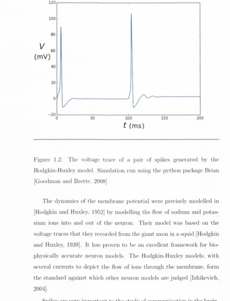
Figure 1.2: Tlio voltage trace of a pair of s]:>ikes generated by the

Hodgkin-Huxley model. Sim ulation run using th e python package Brian

[Goodman and B rette, 2008]

T he dynam ics of the mem brane jioteutial were j)recisely modelled in

[Hodgkin and Huxley, 1952] l)y modelling the How of sodium and jjotas-

sium ions into and out of th e neuron. Their model was based on the

voltage traces th a t they recorded from the giant axon in a squid [Hodgkin

and Huxley, 1939]. It has j^roven to be an excellent framework for bio-

])hysically accurate nem on models. The Hodgkin-Huxley models, w ith

several currents to depict the flow of ions through the membrane, form

the stan d ard against which other neuron models are judged [Izhikevich,

2004],

su b -th resh o ld flu ctu atio n s a tte n u a te g reatly over spaces as sh o rt as 1 nun. T herefore, spikes a rc th e way in w hich neurons co nn n u n icate w ith o th e r regions th ro u g h o u t th e nervous system . W hile th e re is some v ariation in th e d u ra tio n , a m p litu d e a n d shajjc of actio n p o ten tials, for a single neuron th e y ty p ically ex h ib it a c h ara cteristic voltage tra c e as discussed in [Lewicki, 1998]. T h e spike th e n can be rep resented i^y choosing a ])articu lar j)oint of th e ty pical actio n p o te n tia l. T hus, th e tim in g of th e spikes give m uch of th e in fo rm atio n [Bi an d Poo, 1998; B air, 1999]. So, if a neu ron sj)ikes n tim es in a c e rta in trial, th e n th e tria l can be descril)ed by th e tim in g s of th e sjjikes f,. T h e spike train can th e n b e expressed m atliem atically as:

T h e S here is th e D irac d e lta functio n c en tred at f,, w hich has a volum e ('qual to one a t th e p oint

1.2

Spike tr a in m etrics

W hile observ in g sj)ike tra in s from a sj)ecific neuron, ideally one would be able to ‘d eco d e’ th e m and b e able to describe th e stin nilu s which p ro d uced them . T h is ])robleni is very difficult, p a rticu la rly w hen looking at neu ro ns in vivo, th a t is, in living an im als [Averl)eck et al., 2006]. T h ere te n d s to be a lot of noise from o th e r neuron s in th e netw ork which can obscure th e signal to be rep ro d u ced [Hopfield. 1982]. A first stej) which can be ta k en to w ard s solving th is problem is to tr y to distinguish which sj)ike tra in s am o ngst a collection sh are th e sam e stim ulus. T here are several m etrics in th e lite ra tu re w hich give a m easure of th e distan ce betw een i)airs of sjjike train s.

In M a th e m a tic s a m e tric sjiace is a space e(iuipi)ed w ith a scalar fun ction w hich gives a d ista n ce l)etween tw o elem ents in th e s])ace. T he

function is callcd a nictric if it is a scalar function on a set

X , d : X x X

[0, oc) th a t has th e properties a distance niiglit intuitively be ex'pected

to have. T h a t is, distances are non-negative, synnnetric and only zero

if two elem ents are the same. The final proj^erty is called the triangle

inequality, which is a rule th a t ensures the shortest distance between two

points is a straight line.

1.2.1

V icto r-P u rp u ra m etric

In [Victor and P u rp ura, 1997] a family of metrics are described. All th e

m etrics are a tyj^e of m etric called ‘edit-length’ metrics. An edit-length

m etric is based on a theoretical ‘cost' of transform ing one j)oint in a

space to another via elem entary transform ations. T he j^rinciple is th a t

each transform ation has a non-zero cost, so th e distance between two

spike train s can be m easured by minimising the cost to transform one

s])ike train . A", into another,

Y. If zero-cost transform ations are allou'ed,

then such a m easure is a i)seudonietric rath er th a n a metric.

There are three different perm itted fundam ental transform ations. It

is possil:)le to insert a spike at any time, which has a cost of one. Similarly,

any spike can be deleted for a cost of one. The th ird perm itted transfor­

m ation is to move a spike

At .

which ha.s a cost

qAt ,

for some tim escale

p aram eter

q > 0. Formally, the V ictor-P urpura distance between spike

train s is only a m etric when the timescale param eter is positive,

q > 0,

bu t th e

q — 0 case is included in [Victor and P u rp u ra, 1997] to illustrate

the boundary conditions of th e nieasme, and so th e V ictor-Purpiu'a dis­

tan ce is actually a pseudonietric.

sots a n iaxiniuiii tiiiio-franie for tra n sp o sitio n s a t 2 / q . T herefore, given two spikes, /„ in A' a n d ti, in V':

It follows th a t as q te n d s tow'ards zero, it becom es cheajier to move spikes th a n in sert an d delete th em . In th e ca.se w hen q = 0, it costs n o th in g to move s])ikes, th u s th e m easure is equal to th e difference in th e num ber of spikes in A" a n d

T h e n th e V ic to r-P m i)u ra m etric betw een two spike train s, A' and is defined to b e th e m inim um over all co m binations of fund am en tal functions w hich tra n sfo rm A' to T h e m etric can bo w ritte n a.s:

w here f = f \ o . . . o /,„ is a fu n ctio n such th a t / ( A ) = V.

T h is is d e m o n stra b ly a m etric. T h ere is a non-zero cost for each tra n sfo rm a tio n , so d ( X A ' ) = 0 only if A’ = V. D ue to th e fact th a t insertio n an d deletio n are sy n u n etric w ith each o th e r, and transi)osition is a sy m m etric o jieratio n , it is clear th a t d { X . V ) = f/(V, A'). T h e trian gle eciuality follows, since if / tran sfo rm s A' to an d g tran sfo rm s V to Z. th e n It = g o f n m st tra n sfo rm A' to Z , an d sincc th e \^icto r-P uri)ura m etric req uires th a t th e m in in u u n cost, h nm st have cost g re a te r th a n or ecjual to r/(A', Z ).

1.2.2

van R o ssu m m etric

T h e m etric proj)osed in [van R ossum , 2001], is based on th e m etric on function spaces. T h e m etric betw een squ are in teg rab le functions,

f . g . is th e sq u are ro ot of th e in teg ral of th e difference betw een / and g 2 \ta - ^1 > 2 / q

(1.2)

squared, tliat is:

l l / - f ? l l 2 = W ^

(1.4)

(a)

0.02

0.04

0.06

0.08

(b )

0.1

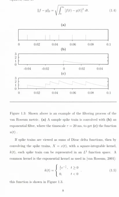
Figure 1.3: Shown above is an example of the filtering process of the

van Rossuni metric, (a ) A samj)le spike train is convolved with (b ) an

exponential filter, where th e tiniescale r = 20 ms, to get (c) the function

If spike train s are viewed as sums of Dirac delta functions, then by

convolving th e spike train s. A' = x(f), with a square-integrable kernel,

each spike tra in can be represented in an

function sj^ace. A

conmion kernel is th e exjionential kernel as used in [van Rossum, 2001]:

1 k { t ) =

t >

0

0.

t <

0

(1.5)

This konicl has th e i)otciitial advantage of causahty over a Gaussian

kernel, and it is very fast to calculate [Houghton and Kreuz, 2012]. Con­

volving th e sjiike train w ith the kernel results in a function, »(/), which

is

measurable:

Figure 1.3 shows the form of the fmiction th a t is produced by con­

volving a si)ike train with tho exponential kernel. T h e metric is then

simply the

L

distance betwet'n these functions:

It has been shown th a t once th e correct tiniescale has been chosen the

choice of kernel has little effect on the perform ance of this m etric [Houghton

and Victor, 2012].

1.3

In fo rm a tio n T h eo ry

Inform ation theory has been used widely in com putational neuroscience,

eg. to comj^are s])ike trains [Strong et al., 1998] and to try to determ ine

th e inform ation content of sj)ike-trains [Gilles])ie and Houghton, 2011].

This thesis uses inform ation theory measures such as the incremental

m utual inform ation [Singh and Lesica, 2010], in Cha])ter Two, and the

tran sm itted information, in Cliaj)ter Three.

The to])ic of inform ation theory is centred around the definition of

entropy, j^rovidc'd by Shannon [1948]. Entropy is a nieasm e of th e infor­

m ation content of a random variable A', with observations

.r £

X

and

probability distribution

p \ X ^

[0,1], it is defined as:

(

1.

6)

(1.7)

H( X ) = - ' ^ p ( x ) log

p{.r)

1

8

Entroj)y is ineasurod in

bits,

so th e entioiw of a random variable can be

viewed as th e minimum numl^er of binary bits recjuired to efficiently code

th e random variable.

To measure the entropy of a spike train a i)robability distribution has

to l)e calculated. In [Strong et al., 1998] a m ethod, which is illustrated in

Figure 1.4, is described to determ ine th is distribution. Each spike train

is binned into a discrete vector of ones and zeros, which indicate w hether

there was a spike in th a t tim e bin. Typically a tim e scale less th a n ten

millisecond in length is chosen for the l)in-size. A larger time-scale,

T,

is

chosen to co n stitu te th e events in the probability sj^ace, which are then

‘w ords’ of ones and zeros. The iM’obability distribution is then calculated

enijjirically from the occm rences of the words throughout th e sj^ike train.

The entropy can be calculated from th e resulting prol)ability distribution.

X

0 | 0 |i| 0 | 0 | 0 | ( ) | ( ) T ( W ' I Q I 1 I 0 I 0 I 0 I ( ) I ( ) I ^ ) | 0 | ( ) | 0 | 0 | 0 | 0 | 1 | 0 | 0 | ^

H

At

T

|0 |0 |0 |l |0 |0 |0 |0 |0 |l |0 |0 |0 |U |0 |0 |0 |0 |0 |( ) |0 |0 |l |( ) |0 |0 |0 |0 |0 |l |0 |0 |

The conditional entropy is a nica^ure of liow much inform ation is in

a random variable A', given th a t th e result of another random variable,

Y,

is known. It is defined:

H{ X \ Y ) = Y . p { y ) H ( X \ Y = y)

y&y

T h a t is, for each value,

y,

of

Y,

th e entropy of

X

is calculated for th a t

set value, then weighted by the probability of th a t value. This can then

be calculated, using Bayes’ theorem:

W(-Y|V') = - V p ( i , ,!/) l o g -

7

The inform ation content of a random variable cannot increase given

knowledge of another variable, so it is always tru e th a t the conditional

entropy,

H{ X\ Y ) ,

is less th an the entropy of the variable itself,

H{ X) .

The difference lietween the two vahies can be viewed as the shared infor­

m ation of th e two variables. The

inutunl information

of two variable is

defined as:

■rex.y^y ''

: i . i i )

which can equivalently be expressed as:

7(A';r)

=

H[ X ) - H[ X \ Y ) = H{ Y) - H( Y\ X) .

(1.12)

If two varial)les are inde])endent, then the joint distribution of A'

and

y would be equal to the product of th e m arginal distributions, and so

thev would have zero m utual information.

1.4

D a ta sets

The spike train m etrics in this thesis wore tested on d a ta sets to suit the

experim ent th a t was undertaken. W hile an effort was made to use real

electrophysiological d ata, some ex])eriments recjuired the use of sim ulated

data.

1.4.1

Zebra finch d a ta

Single neuron spike train m etrics, in C hapters Two and Four of this

thesis, were tested on the d a ta set used in [Narayan et a l , 2006]. The d ata

set was obtained by inserting an electrode into the auditory forel)rain

of anaesthetised zebra finches and recording th e neuronal responses to

m ultiple presentations of conspecific song stimuli. The fact th a t the birds

were anaesthetised m eans th a t there would be minimal feedback to the

neiu’cns in th e forebrain from other brain fimctions.

T here were recordings from 24 such cells. Each cell was presented

w ith 20 separate songs ten tim es each, as shown in Figure 1.5, w ith a

tone to signify th e sta rt of th e recording precisely one second before the

onset of th e stim ulus.

Zebra hnch d a ta is of p articu lar use in C h ap ter Four, as there is

evidence of feature recognition in resjionses to n atu ral songs in the zebra

finch forebrain [Sen et al., 2001]. C hapter Four introduces a simple model

of firing which would be consistent w ith sparse coding. D ata sets with

highly tem poral features are thus im p o rtant in testing the model.

1.4.2

M u lti-u n it d a ta

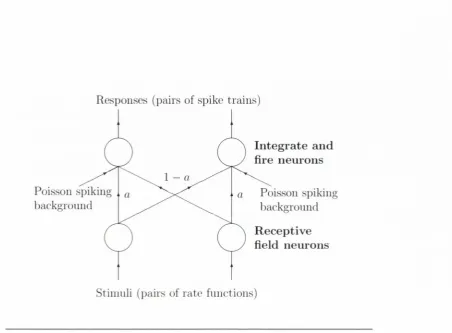
The m ulti-unit distance m easures in chapter three were tested on the

same sim ulated test d a ta as in [Houghton and Sen, 2008]. Two Pois-

son neurons form a receptive field and are each connected to two leaky

integrate-and-fire neurons (LIF) w ith relative stren g th

and 1 — a;

is

called th e mixing param eter of th e sim ulation. \M ien

0 each recep­

tive neuron is connected to a single LIF neuron, and for

= 0.5, each

LIF neuron receives input equally from each of the receptive neurons.

M

F igure 1.5: T lie d a ta used w as collected for [N arayan et al., 200G]. A to ta l of 20 songs were played to a n ae sth etise d zel)ra finches, a n d th e responses were recorded in th e au d ito ry forel)rain. Each song was presen ted ten tim es. R esponses of th re e different cells to th e sam e song are shown lier('.

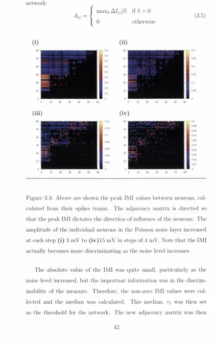
confusion m a trix is calcu lated whoso entries N i j represent th e nu m ber of responses from stin n ih is i which are closest, on average, to th e resjjonses from stim u lu s j .

Tlie tra n s m itte d inform atio n, h , is th e n calcu lated from th e confusion m a trix . A’.

I) = — ^ A y I hi N. jj — hi ^ N , j — hi ^ N j j + hi ??

j

V \ i j /

W’liilo it may be jircfciable to test m etrics on biological d a ta in most

cases, it is crucial to comi^are th e perform ance of th e m ulti-unit metrics

w ith a controlled mixing param eter. The d a ta presented here allows an

analysis of th e m ulti-unit m etrics’ perform ance as the data varies from

R esponses (p airs of spike train s)

Integrate and

fire neurons

Poisson spiking backgrouncl

Poisson spiking background

R ecep tiv e

field neurons

Stinnili (])airs of ra te functions)

F igu re l.C: T his is th e schem atic for th e d a t a set used to te st th e m ulti- im it m etrics in tliis thesis. It is th e sam e d a ta set th a t was used in [H oughton a n d Sen. 2008]. T he receptive field neurons fire Poisson spike tra in s according to th e r a te fun ctio n in p u t th e y receive. T hese Pois­ son sj)ike tra in s feed into th e leaky in te g ra te a n d fire (L IF ) neurons from w hich th e response is m easured. T h e sy n a p tic s tre n g th s are i)aram etrised by a m ixing ])aram eter a. W hen a is zero, th e LIF neurons receive inde­ p en d en t ini)ut; w hen a = 0.5. th e in p u t sho uld be identical.

Chapter 2

C lustering m ethods in spike

train analysis

Tliis chapter ai)i)roaclies iieuroscieiice from th e point of view th a t there

are clearly functional connections between neurons in th e same region of

th e brain and th a t these connections could provide a m ap of information

flow in the brain. Comi)lex network theory, a l)ranch of m athem atics

closely related to grajih theory, is used frecjuently in coni])ntational neu­

roscience.

Comi)lex networks often exhibit a connnunity stru ctu re, and so there

are many algorithm s to find the best clustering of a given network [Karypis

et al., 2000; Newman and Girvan, 2004; Newman, 2006a]. This cha]:)ter

introduces the clustering algorithm developed by Newman [2006a], and

suggests some new algorithm s l)a.sed on the m odularity m easure [New­

man and Girvan, 2004]. These new algorithm s are based on complexity

algorithm s, genetic algorithm and sim ulated annealing, which recjuire

nothing more than a ‘goodness-of-fit’ function. Com plexity algorithm s

often produce interesting results, a.s they do not take a i)re-determined

j)ath through th e solution space.

Newm an's algorithm [Newman, 2006a] is then used to cluster neuron

responses dynam ically, w here th e nu m b er of stim uli need not be known.

A netw ork of responses is form ed by co m p aring th e van R ossum d istan ces

l)ctwoen th e sj)ike train s, an d th e n choosing a d istan ce th resh o ld w here

an y d ista n c e less th a n th e th resh o ld form s a link. By clu sterin g th is

netw ork using th e eigenvalue alg o rith m of N ew m an [2006b], it is not nec­

essary to specify th e num l)er of stim uli in advance, unlike th e connnonly

used m eth o d s, A’-m eans an d /.--medoids.

2.1

In trod u ction to netw orks

C om plex netw ork th eo ry differs from g rap h th e o ry in th a t it focuses

on th e tr a its th a t netw orks te n d to have w hen th ey evoh'c in real hfe,

r a th e r th a n focusing on pu rely ran d o m netw orks. T h e m ain difference

betw een th ese w ould be th e co n n ectiv ity profile of th e netw ork: in g rap h

th e o ry connections are usually sp read .somewhat uniform ly th ro u g h o u t

th e g rap h , w hereas in N etw ork T h eo ry it is ex])ected th a t com m unities

w ould form [Newman. 2010].

A m a th e m a tic a l netw ork is simi)ly a collection of nodes an d links

betw een th ese nodes. A node is sim j)ly a ])oint in th e graj)h. w hich is

ty p ically discrete a n d labelled. A link is a p air of nodes w hich ind icates

a connection betw een th e two nodes. T h e degree of a node is defined to

be th e n um ber of links incident to th e node. An m idireeted n etw ork w ith

n no d es can be com pletely described l)y its adjacen cy m a trix A w here

Aij = 1 if nodes i an d j are connected, a n d is equal to zero otherw ise. In

th is case A,j = A ji since tw o nodes are e ith e r conn ected or no t. If m a trix

en tries A jj are i)ern iitted to ta k e values o th e r th a n one an d zero th e n

th a t is called a weighted netw ork. A netw ork is called a directed netw ork

if = 1 w henever th e re is an arrow jx)inting from nod e j to node i, an d

th e adjacency m a trix is not necessarily sy n n n etric. U n directed netw orks

lioher in tliis ease. A ioa.son for th is could be tlia t netw orks snch a.s friend

netw orks [Zachary, 1977] w ould ty])ically not l)o d irected as friend ship is

ty])icaiiy m utual.

A ])articularly in terestin g j^art of netw ork th eo ry tlia t could l)o useful

for neuroscience is clustering, an d algorith m s to m axim ise th e co m m u n ity

s tru c tu re of th e clusterings. To m axim ise th e co n u n u n ity s tru c tu re , a

n ieasm e of such s tru c tu re is reciuired.

2.2

M od u larity

T h e modularity is a m easure of a given clu stering of a n etw ork, w hich

gives a value to th e con n n u n ity s tru c tu re of th e clu stering [Newm an an d

G irvan, 2004]. T h e m o d u larity is defined to m easure how m uch m ore

jjrom inent in tra-clu ste r links are th a n in ter-clu ster links in a given clus­

tering. T h e m o d u larity th en , as a m easure of th e given clusterin g, m ea­

sures how much co n u n u n ity s tru c tu re is seen in th e netw ork. It was

intro d u ced by N ew m an and G irvan [2004] in one form, th e n N ew m an

[200Ca,b] derived a n o th e r form using th e configuration m odel for grai)hs

[Bender and Canfield, 1978: Bollobas, 1980].

T h e m o d u larity is a m easm 'e of a clu stering of a netw ork th a t assesses

how nm ch m ore con n n u n ity s tru c tu re th e re is in th e netw ork th a n th e re

w ould b e in a rand om netw ork w ith sim ilar proj)erties. In [Newman,

2006a,b] th e m o d u larity is derived as follows in th is section. T h e m o d u ­

larity is defined to be th e difference betw een actu al links w ith in clusters

an d th e expected nunil)er of links. Sum m ing over all nodes w ith in a

clu ster, g\

(Links in g) — (E x p ected links in g) = A^j — P,j (2.1)

w here Pjj is th e ])robability of a link l)etweeii nodes / an d j . T h en , if

g, is th e com m unity to w hich node / belongs, th e m o d u larity Q can be

F igu re 2.1: T h e ad v an tag e to clu sterin g a netw ork co rrectly can b e seen

here. Shown are tw o d iagram s w hich have th e sam e nodes an d links,

an d so form th e sam e netw ork, b u t th e y look vastly different because th e

d ia g ra m on th e left h as been clu stered to m axim ise m odularity.

described:

w here ^ is th e K ronecker d elta, so S i g i . g j ) = 1 if nodes i and j are in th e

sam e cluster, a n d zero otherw ise, m is th e to ta l m u nb er of links in th e

netw ork, and so l/2?r? is ju s t a norm alising factor. T h e m o d u larity of a

clu ster is th e n th e n u m b er of edges w ith in a clu ster m inus th e exp ected

n u m ber of edges.

N ew m an [2006a,):)] calcu lates th e p ro b ab ility of a link l)etween nodes

in th e configuration m odel. In u n d irec ted netw orks, clearly th e p ro b a ­

bilities should b e sym m etric, Pjj — Pji. T h en , th e ex pected nu m ber of

links across th e w hole netw ork should ecjual th e to ta l n u m b er of links.

w here iti, as before, is th e to ta l n u m b er of edges in th e netw ork, so if th e (2.2)

T h a t is, - Pij] =

At th is ])()int, th ere is som e choice as to how siniihir th e raiicloiu

netw ork, th a t th e calcuhited p ro b aliih ties are l)ased on, sh ould be to th e

netw ork itself. O ne could su pp ose th a t each node in th e ran d o m netw ork

has degree equal to th e average degree of th e netw ork, b u t th is ignores

local s tru c tu re in th e netw ork. In stead , it is supposed th a t th e rand om

netw ork should keej) th e sam e degree for all nodes, a n d so th e netw ork

can be tre a te d as an in stan ce of th e configuration model [Bender and

C anfield, 1978; Bollobas, 1980]. So, th e ex p ected degree of each vertex

is e(}ual to th e a c tu a l degree of th e vertex:

If it is supposed th a t beyond th e degree d istrib u tio n th e edges are

placed at ran do m , th e n th e p ro b ab ility of two nodes co nn ectin g dejiends

on th e ir degrees. Sui)posing th e p ro b ab ilities for each end of a single

edge is ind ejjcndent, w hich is a reaso nable assum i)tion in a large netw ork

[Newman, 2010], w here all th e degrees are sm all relative to th e to ta l

nu m b er of edges, P,j = f ( k , ) f { k j ) for som e function / on th e ir degrees.

T h en , by eq u atio n 2.5:

(2.5)

J

n

j = i j = i U = i

so f{k'i) — Ck'i, for som e co n stan t C , a n d we get

(2.7)

an d th e m o d u larity is

(2.9)

T h e m o d u larity gives vahies l)ctween —1/2 an d 1 for any clustering. Since it is know n th a t n ot d ividing th e netw ork into sej^arate clusters gives a m o d u larity of zero, th is gives us a lower b o u n d for “good” clus­ terings.

T h e benefit of finding a good clustering can b e seen in figure 2.1; a good clu sterin g can reveal w h at th e n a tu re of th e netw ork is, ra th e r th a n it being a m ess of nodes an d links. W hile th e m o d u larity itself is a m easure of a given clusterin g of a netw ork, th e m axim um m o d u larity is a p ro p e rty of th e netw ork itself, w hich can tell much ab o u t th e in­ herent co n n n u n ity s tru c tu re of th e netw ork. To actu ally d eterm in e w hat clu sterin g will give th e m axim um m o d u larity a n ex h au stiv e search would be recjuired, w hich becom es mifea.sible for netw orks of even a m o d e ra te size, as th e nu m b er of p o te n tia l clu sterin g s is huge. T herefore, clu sterin g alg o rith m s are needed to m axim ise th e m o d u larity of th e netw ork.

2.3

N e w m a n ’s eig en v a lu e a lg o rith m

In [N ewm an. 2006b,a] N ew m an n o te d th a t if it was sujijjosed th a t th e netw ork was si)lit into tw o clusters, th e n th e m o d u larity could b e rede­ fined in te rm s of a q u a d ra tic form. D efining a v'ector s, w hich keeps track of th e split.

— 1 if n o d e i in ch ister 2

T h ese vectors .s,: th e n co n tain th e exact sam e inform atio n as th e 2 x ?? m a trix S { g i , g j ) , so S { g i . g j ) can b e factored:

1 if n o d e i in clu ster 1

(

2

10

T h en , th e m o d u la rity is redefined a.s:

(2.12)

Let B l)e a m a tr ix w here Bjj = Aij — k j k j / 2 m , called th e modularity

matrix, th e n e q u a tio n 2.12 l)ecomes:

Q = — s *B s (2.13)

i n i

Now , since B is an n x v s y n n n e tric m a trix , it has v real eigenvalues

Ai, w ith co rre sp on d ing eigenvectors u,. O rd e rin g th e A, so th a t Ai >

A2 > .. ■ > A „. th e n w rite

so, th e ])o s itiv ity o f th e m o d u la rity depends c o n i])le te ly on th e A,, in

])a rtic u la r th e m ost j)o s itiv e eigenvalue A i. T h is means th a t to n ia x -

inii.se th e m o d u la rity th e “ s j)lit v e c to r” s o u g h t to be a.s close to th e firs t

eigenvector U i as possible. To do th is , choose s as follow s:

T h is gives a c lu s te rin g o f th e n e tw o rk in to tw o sm a lle r clusters. O f

coiu’se, th is s p lit is n o t s t r ic tly in th e d ire c tio n o f A i, b u t it is th e best

])ossible e stim a te , given tw o clusters. In fa c t, it ha.s been noted fro m w e ll-

kn ow n netw orks, such as Z a c h a ry ’s karate c lu b [Z achary. 1977], w here

friend.shi])s w ith in a k a ra te c lu b w vre grai)hed j)rio r to th e c lu b s j^ littin g , s = f / iU i + .. . + r;„U n (2.14)

T h e e q u a tio n fo r th e m o d u la rity becomes

Q

J

(2.15)

1 i f Ui > 0

11

- 1 i f ( / i , < 0

(2.16)

th a t th e ab so h ite vahie of th e /th en try of u i gives a good inchcation of tlie “stren g th " of th e m em bersh ip of node / to its ch ister [Newman, 2006b], T h a t is, an e n try ui , i w ith ab.sohite vahie close to one can be observed to be a key in tra -c lu ste r no de or hub. In th e case of Z achary's k arate club th ese in tra -c lu ste r hubs were th e different in stru c to rs who split th e club into two clubs.

If th e m o d u larity of th e split is n ot positive, th e n reject th e sj^lit and say th a t th e b e st clu sterin g is to leave th e netw ork as it is. Sim ilarly, if th e first eigenvalue Ai = 0 th e n say th a t th e )>est clu sterin g is to leave th e netw ork m idivided, as it is know n th a t th e m o d u larity m a trix B always has a zero eigenvalue, w ith eigenvector u = ( 1 , 1 , . . . . 1 ) . which corresj)onds to no split of th e netw ork.

W ith th e netw ork split into tw o sm aller clusters, th e next questio n is how to sj)lit th e netw ork fu rth er. X ew m an [Newm an, 2006b] recom m ends looking at th e clusters one-by-one a n d sp littin g th e m u n til it gives no benefit to th e m o d tilarity of th e overall clustering. O ne could naively ju st look a t th e ad jacen cy m a trix of th e clu ster itself, an d form th e correspo nd ing m o d u la rity m a trix , b u t th is ignores th e co nn ectiv ity of th e overall netw ork. T h a t m eth o d could in a d v erten tly sj^lit th e su b g rap h into co m m u nities w hich would m ake sense w ith in th e clu ster, b u t would ignore th e conn ectio ns from o u tsid e th e cluster. In stead , th e original m o d u larity m a trix B is used to calcu la te w h a t difference a split of th e su b g rap h w ould m ake to th e m odularity.

G iven a clu ster of n odes g, w ith in th e netw ork, th e m odularity con­ tribution A Q of a split of g is;

T h is is th e te rm in th e m o d u larity of th e netw ork th a t a sjjlit s of g w ould change, m inus th e m o d u la rity of leaving th e su b g ra p h g whole. T hu s, a

“subgTai)li in o d u la iity m atrix”

can be defined as:

L

(2.18)

and so

takes the value

b “ = By -

(2.19)

for labels i , j of nodes in the cluster g.

The

th e

the j^roperty th a t each of its rows sum to zero, so there still is a z e ro

eigenvalue th a t represents no si)lit of the cluster. This can now be the

stopping criterion for th e algorithm ; if the most positive eigenvalue is

th e zero-eigenvalue, then th a t subgrai)h is indivisible and stoj) si)litting.

It should be noted, however, th a t as the most positive eigenvalue gets

smaller, relative to its negative eigenvalues, th ere may he no benefit to

th e m odularity of accei)ting such a sj)lit. In this case chec'k, by calculating

A Q

for the proposed sjilit, to see if it is w orth c‘ontinuing splitting the

subgraph. If

< 0 then stop, otherwise continue si)litting the graph.

The algorithm is sum m arised in Algorithm 1.

This eigenvalue m ethod for maximising th e m odularity has shown re­

m arkably good results [Newman, 200Gb], despite the apparent drawback

of always splitting th e netw ork/subgraph in two jiarts. It is ])ossil)le to

sj^lit th e network into more th an two p arts initially by using the first

tri

eigenvalues and using the ith entry of the eigenvectors as coordinates

in R "' [Hunii)hries, 2011], but this then requires a choice of num ber of

A lg o r ith m 1 This is N ew m an’s cigcnvahie algorithm for maximising the

m odularity of a network.

C alculate th e m odularity m atrix B , where

Dij = A,j — kikj/2iv

Find the most positive eigenvalue Ai and its eigenvector Ui

if Ai = 0 t h e n

Stop th e algorithm w ith no split in the network.

e lse

Split network such th a t node

i

in first group if

ui- >

0 and in second

group otherwise.

E n s u r e :

M odularity of split > 0

e n d if

fo r a ll subnetworks

g

d o

C alculate

where

Find th e most positive eigenvalue

of

and its eigenvector

if Aj''^ = 0 t h e n

Subnetwork can split no further,

e lse

Split network such th a t node

i

in first group if

>

0 and in

second group otherwise

E n s u r e :

A Q >

0 for s])lit of sul^network

g.

e n d if

large m atrix B , which can be coniiMitationally expensive, rath er th an

calculating a single eigenvalue for smaller and sm aller m atrices as above.

2.4

N ew netw ork clu sterin g algorithm s

Using the definition of m odularity as defined above in equation 2.9 to

measure the connnunity stru ctu re of given clusterings, two new algo­

rithm s were developed in the covu’se of this thesis. They both use com­

plexity algorithm s, which can often find novel solutions to difficult prob­

lems, since they do not make assum ptions about the natiu'e of th e solu­

tions.

2.4.1

G e n e tic algorithm

Genetic algorithm s have l^ecome widely used to .solve complex o})timisa-

tion jHoblems where it is difficult to calculate the gradient of the objective

function. The algorithm is based on the process of Darwinian evolution

where successful genes rem ain in the gene pool and unsuccessful genes die

out. Tliere have been several clustering algorithm s which use the genetic

algorithm as their framework, such as [Pizzuti, 2008]. In this projjosed

algorithm the genes are sinq)ly the clusterings of a given network and

th e m odularity is then the objective fmiction.

The sinq)licity of a typical genetic algorithm is th a t it tyi)ically only

needs a fitness/objective fimction to evaluate the fitness of solutions. A

genetic algorithm is (lescril)ed in A lgorithm 2.

To define a genetic algorithm , it is inq jo rtan t to define w hat a solution

is, and how th e genes crossover and m utate from generation to generation.

In this case, a solution is any clustering of the netw’ork. A fitness function

is a function of .solutions which should tyi)ically be non-negative. This

can be attaine'd l>y setting the fitness of any clustering with negative

A lg o rith m 2 An example of a generic genetic algorithm.

Generate a random population of

n

genes

gi,

set generation to zero.

w hile Generation <

N

do

for all Genes

do

Calculate the fitness of

g,.

e n d for

Breed new population:

for

i

}. do

Choose parents according to goodness-of-fit.

Generate new gene

gi

by crossover of j^arent genes.

M utate

gi

with probability f.

e n d for

for all

gi

d o

(h < - gi

e n d for

m o d u larity to zero, b u t since th e lower bo u n d is sh a rp it is b e tte r to use

th e m o d u larity plus 1 /2 as th e fitness function. / . T h en a clu sterin g </,

is chosen as a p aren t w ith p ro b ab ility /{(]]))■

It is im p o rta n t to m a in tain asj)ects of th e “p a re n t” genes w hen b reed­

ing th e new genes; th e n um b er of clu sters is a very in ij)o rtan t asp ect of a

clustering, so any alg o rith m m ust b e careful not to sim i)ly crossover clus­

terings by tak in g th e ir in tersection as th a t w ould ty pically increase th e

num ber of clusters. T h e upj^er lioiuid for th e nu m b er of clu sters should

be set to th e m axim um of th e num b ers of clu sters of th e p aren ts, or by

settin g Uc = (» ,/((/,) + n j f i g j ) ) / { f i Qi ) +

Crossover is defined in th is alg orith m by ran do m ly choosing a sin­

gle node in th e netw ork according to th e degree d istrib u tio n , an d th e n

ran do m ly choosing th e clu ster w hich co n tain s th e node in one of th e

p aren ts. Reniove all nodes in th e chosen cluster from th e selection i)ool,

an d continue th e j^rocess. If th e n um ber of clu sters reaches th e predefined

m axim um n um ber of clu sters an d som e nodes rem ain, th e n th e rem aining

nodes are placed in th e closest clu ster to th e m (by p a th d istan ce). M u­

ta tio n is defined by ran do m ly m oving a sm all i)ercentage. ai)p ro xim ately

15%, of nodes betw een clu sters in ap])roxim ately 10% of clusterings.

T his alg orith m is c(jm pu tationally very exjicnsive for sm all netw orks,

))ut scales nm ch b e tte r th a n N ew m an ’s eigenvalue alg orith m .

2.4.2

S im u lated an n ealin g

A n o th er algorithm from coni])lexity th e o ry w hich has previously been

used for finding co n n n u n ity s tru c tu re in netw orks is sim u la ted annealing.

S innilated an nealin g is an alg o rith m based on th e techni(iue of ann ealin g

in m etallurgy; an nealing h ap p en s w hen a m etal is heated an d th e n cooled

slowly to increase th e size of th e cry stals in th e m etal, as th e m etal finds

th e cry stal s tr u c tin e w hich recjuires lowest energy as it cools slowly.

Siinulated annealing mimics this process to find a solution th at min­

imises an

energy

function, by introducing a

temperaiure

of sorts to the

system. At each tem perature level, there is a small change to the solu­

tion, and the new energy level is calculated.

The i)robability of accepting the change to the solution is then de­

termined by an

acceptance probability function, P{E{s), E{s' ),T),

which

depends on the cm-rent energy

E{s),

the potential new energy

E{s')

and

the tem perature

T.

The basic rule of the algorithm is th at any change

of state th a t reduces the energy of the system is automatically accepted,

and a change of state th at increases the energy is accepted with a j^rob-

ability th at decreases as T —)• 0.

The accej)tance probability function used also has the ])roi)erty that

small increases in energ>^ are more likely to be accepted than liig increases

in energy. The acceptance probalnlity is then a decreasing function of

the change in energy

A E

=

E{s') — E(s),

which decreases faster as the

tem perature lowers. An exponential fmiction satisfies these criteria:

f

1

E{s') - E{s) <

0

P ( E ( . v ) , £ ( . s O , r ) = . (2.20)

1^ exp

E{s') - E{s) >

0

The solution sj:>ace for this algorithm was the s])ace of clusterings of

a given network A^ The “energy'’ function was the modularity with the

sign reversed.

It is imj^ortant for simulated annealing that all moves are small. W ith

this in mind, the move in this clustering algorithm is simply to select a

node at random and move it to either any existing cluster or to form a

new cluster from it. From observations, this algorithm did not appear

to be very discriminating w'hen required to split a network to more than

two or three clusters, but it did seem to find “stable” solutions. For

example, in Zachary’s karate club network [Zachary, 1977] it found the

correct split of the network, rather than the clustering which resulted in

2.5

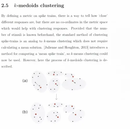
/c-medoids clu sterin g

By defining a metric on spike trains, there is a way to tell how ‘close’

different responses are, but there are no co-ordinates in the metric space

which would help with clustering responses. Provided that the num-

l)er of stimuli is known l)eforehand, the standard method of clustering

spike-trains is an analog to A’-mcans clustering which does not require

calculating a mean solution. [Julienne and Houghton, 2013] introduces a

method for computing a ‘mean sj^ike tra in ’, so A'-nieans clustering could

now l)e used. However, here the process of A-medoids clustering is de­

scribed.

(b)

Figure 2.2: An exanii)le of the first stej) in k-medoids clustering: (a)

Medoids are initially selected at random and the first clustering puts

each point in the cluster of the closest medoid. Then we choose the point

in the cluster that will give the lowest total distance to other jioints, and

choose that as the new medoid. (b) Finally, w'e re-cluster each ]:)oint to

go in the cluster of the closest medoid to it.

For A’-means clustering,

k

random j)oints are selected in the sj)ace in

which clustering is occurring, then each j^oint in the sj)ace would be in

th e ch istcr of th e closest of those k jio in ts to Itself. T h en th e m ean of all

th e p o in ts in a clu ster is calcu lated to get a new •‘cen tre'' for th e cluster

an d re-clu ster each j^oint to th e closest of these k m eans. T his jirocess

is I'ejieated m itil th e m eans are stab le, w hich gives a clusterin g of th e

p o in ts in to k clusters.

T h e A'-medoids alg o rith m begins by choosing a p re-d eterm in ed num ­

ber, k, o f p o in ts in th e d a ta , called niedoids, a n d th e n each o th e r ])oint

of th e d a ta is j)laccd in th e ch istcr of th e closest, or least dissim ilar),

niedoid to it. T h en , for each clu ster, each j^oiiit in th e clu ster is assessed,

a n d th e jioint w ith th e least overall d ista n ce is chosen as th e new niedoid.

T h is step is show n in F igure 2.2. T hese step s are rei)eated u ntil th e re is

no change in th e niedoids. T h is m e th o d su its for s])ike-trains, as th e idea

of a ‘m e a n ’ spike tra in is not well u n d ersto o d , alth o u g h , using th e van

R ossuin m etric, th e average fun ctio n of Ju lie n n e a n d H oughton [2013] is

a possible altern ativ e.

T h ere are som e dow nsides to using A’-niedoids, th a t could jiossibly be

inii)roved by using netw ork m etho ds. T h e i)rim arv d isad v an tag e is th a t

th e n u m b er of clu sters m ust be selected in advance, and hence imi^lies

])rior know ledge of th e nu m ber of different stim uli th a t are jiiesen ted in

a d a ta set. T his is ad dressed in th e next section.

2.6

C lu sterin g resp on ses w ith m od u larity

H ere it is j)roi)osed th a t c u rre n t m e th o d s of so rtin g resi)onses could j)o-

teiitially be im proved by using th e m o d u larity clu sterin g algorithm . An

ad v an tag e to such a dy nam ic m e th o d would be th e ability to clu ster re-

si)onses w ith o u t foreknow ledge of th e stim uli. T h is suggests th a t fu tu re

dyn am ic so rtin g alg o rith m s m ay be possible. Since th e alg o rith m de­

term in es w hen to sto p itself, it is sim ply l)e ru n to com pletion. Such a

iiuinl)er of stimuli was not known, to determ ine the different responses.

The d a ta set introchiced in the introchiction from [Narayan et al.,

2006] was used, which featured sj^ike trains from anaesthetised adult

male zebra finches as they listened to conspecihc songs.

A distance m atrix was calculated by taking the van Rossmn m et­

ric distances between each j)air of responses for each neuron, where the

param eter r in the m etric wa.s chosen to be 12.8 ms, as this had pre­

viously l:)een determ ined to be a good param eter for th e d a ta set used

[Houghton, 2009]. Then, given a threshold value, //, th e adjacency m atrix

for a network was calculated as:

Once th e adjacency m atrix was calculated, th e algorithm was run

to maximise m odularity for the network. T he nuiximum van Rossuui

distance, once normalised, between any two train s was one, so the al­

gorithm was run for different threshold values // between zero and one

increm enting // by stej)s of size 0.001.

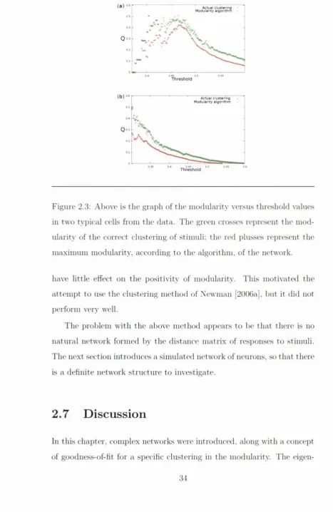
As seen in H gure 2.3. th e profile of the graph of th e m aximum mod­

ularity versus the threshold looked j^romising. as for each cell th e mod­

ularity peaked as // varied, but unfortunately th e clusters of responses

bore little resenil)lance to the stinuili, and usually had too few clusters.

D('spite there being clear i)eaks in the m odularity grai)hs, th e maximised

m odularity consistently outi)erfornis the m odularity of the correct clus­

tering for every value of the threshold //. This sc'oms to im])ly th a t n et­

work clustering m ethods are ])robal)ly not very good for sorting stinmli.

The m odularity m axim isation of these networks unfortm iately cannot

cluster the responses by their stimuli. A sim ilar m ethod was used in

[Humphries, 2011], where all of the positive eigenvalues were u.sed to

cluster responses, . This m ethod is rath er com putationally exi)ensive,

and uses even the very small ])ositive eigenvalues, which themselves may

0 otherwise

1 i f f / ( / , j ) < / /

(2.21)

0 6

a A c tu a l c lu s te r in g M o d u la rity a lg o r ith m

0 4

Q0 3 0 3 0 1

0

0 4 OS 0 55

( b ) « » A c tu a l c l u s t e n n g M o d u la rity a l g o r i t h m OS

0 4

0 2 0 1 0

0 35 0 4 0 45 0 5 0 55 0 6

T h resh o ld

Figure 2.3: Above is th e graph of th e m odularity versus threshold values

in two typical cells from the data. The green crosses represent the m od­

ularity of the correct clustering of stimuli; the red j:)lusses rei)resent the

m axim um m odularity, according to the algorithm , of the network.

have little effect on th e positivity of m odularity. This m otivated the

atte m p t to use th e clustering m ethod of Newman [2006a], but it did not

pcnform very well.

The problem w ith th e al)ove m ethod a])i)ears to be th a t there is no

n atu ral network formed by th e distance m atrix of responses to stimuli.

The next section introduces a sim ulated network of neurons, so th a t there

is a definite network stru ctu re to investigate.

2.7

D isc u ssio n

In this chapter, complex networks were introduced, along w ith a concej^t

eigen-value algorithm introduced by Newman [2006a] w^as introduced in detail,

a.s it has become the l^enchmark for clustering algoritluns.

Two new algorithm s w'ere introduced to try to find a clustering th at

would maximise the m odularity of a network. N either ])roducecl results

l)cttcr th an the stan d ard m ethods, so were used sparingly. The sim ulated

annealing algorithm appeared to not necessarily maximise th e m odular­

ity, bu t seemed to find the highest ‘stable’ modularity.

Netw'ork m ethods did not cluster stim uli w^ell, perhaps because the

network stru ctu re was not natural. This may rule out network clustering

m ethods as a tool for discrim inating betw^een responses, but [Humi)hries,

2011] seemed to get results w ith a different d a ta set, so it is not conclu­

sive. The sinuilated annealing algorithm introduce in this chapter could

potentially provide interesting clusterings of stinuili, b u t th a t was not

ex])lore(l in the work for th is thesis.

The dynam ic response clustering aj^jieared not to work due to a lack of

network stru ctu re am ongst the resjjonses. The next chaj)ter thus focuses

on a sinm lated network of neurons w ith known netw'ork structure. This

appears to be th e optim al w'ay to use network clustering in neuroscience.

I I

C hapter 3

M apping inform ation flow in a

sim ulated netw ork o f neurons

In this chai)tcr, a process is i)roj)osed for a way to m ap how inform ation

flows througli a network of neurons. T he process is proposed due to the

ol)servation th a t given an inter-si)ike inter\'al (ISI) distribution which

arises from a neuron liaving a refractoriness after each sj)ike, such a.s

th e gam m a function or the inverted normal (hstribution, then a very

small grouj) of neurons, say 20 to 30, is sufhcient for the collection of

neurons together to jiroduce an exponential distribution of ISIs - which

would be the ISI distribution of a Poisson rate jHocess. Due to this

observation, it is proi)Osed th a t there should be small clusters of neurons

th a t work together to ])rovide a background ‘ra te ’ to other sim ilar groups

of neurons.

There are different ways to form th e networks of many neurons, but

of i)riniary interest are neurons whose firing seems to improve the prob­

ability of other neurons hring. A m ethod of particular interest is the

m ethod of

Incremental M utual Inforina.tion

of Singh and Lesica [Singh

and Lesica, 2010], which tries to reduce the uncertainty of a neuron as

much a.s possible before checking w hether another neuron influences it.