R E S E A R C H
Open Access
Optimal investment of a time-dependent
renewal risk model with stochastic return
Jiesong Zhang
1,2*and Qingxian Xiao
1*Correspondence:
1Business School, University of
Shanghai for Science and Technology, Shanghai, 200093, China
2School of Mathematical Science,
Huaibei Normal University, Huaibei, 235000, China
Abstract
Consider an insurance company which is allowed to invest into a riskless and a risky asset under a constant mix strategy. The total claim amount is modeled by a non-standard renewal risk model with dependence between the claim size and the inter-arrival time introduced by a Farlie-Gumbel-Morgenstern copula. The price of the risky asset is described by an exponential Lévy process. Based on some known results, the uniform asymptotic estimate for ruin probability with investment strategy is obtained with regularly varying tailed claims. Applying the asymptotic formula, we provide an approximation of the optimal investment strategy to maximize the expected terminal wealth subject to a risk constraint on the Value-at-Risk, which is defined with respect to finite-time discounted net loss. A numerical example is illustrated for the results, which demonstrates that big dependence parameter is advantageous for the insurer. We explain the reason by some inequalities.
Keywords: dependence; optimal portfolio; Lévy process; asymptotics; Value-at-Risk (VaR)
1 Introduction
The renewal risk model has been playing a fundamental role in classical and modern risk theory since it was introduced by Sparre Andersen in . In this framework, the suc-cessive claims{Xk,k≥}form a sequence of independent identically distributed (i.i.d.)
random variables (r.v.s), and their inter-arrival times{ξk,k≥} form another sequence
of i.i.d. r.v.s, and the two sequences are mutually independent too. However, the inde-pendence assumption between the claim sizeX and the inter-arrival timeξ is too re-strictive and sometimes unrealistic in many kinds of insurance. HereX and ξ denote the generic r.v.s of the claim sizes and inter-arrival times, respectively. In fact, for a line of business covering damages due to earthquakes, more quantities of damages are ex-pected with a longer period between claims, since the claim amount (or the intensity of the catastrophe) and the time elapsed from the previous one are assumed to be pos-itively related by the seismic gap hypothesis (see,e.g., Nikoloulopoulos and Karlis [] and Boudreaultet al.[]). Furthermore, the period between claims must be longer if the de-ductible of the insured increases, since some of the small claims will not be considered. During the last decade, initiated by Albrecher and Teugels [], many scholars have started to propose some non-standard renewal risk models with various dependence structures. Among them, Albrecher and Teugels [] considered that (X,ξ) follows an arbitrary de-pendence structure based on a copula, and they derived explicit exponential estimates for
finite- and infinite-time ruin probabilities. Cossetteet al.[] assumed a generalized Farlie-Gumbel-Morgenstern (FGM) copula for (X,ξ), and they derived the Laplace transform of the Gerber-Shiu discounted penalty function. Bargèset al.[] derived the moments of the aggregate discounted claims with dependence introduced by a FGM copula and the count-ing process followcount-ing a Poisson process. Asimit and Badescu [] described the dependence structure via the conditional tail probability ofXgivenξ, and they studied the tail behav-ior of discounted aggregate claims in the Cramér-Lundberg risk model in the presence of a constant force of interest and heavy-tailed claim sizes. Yong and Xiang [] obtained an integro-differential equation for the expected discounted penalty function with a FGM copula betweenXandξand the distribution ofξ being a sum of two independent expo-nential r.v.s.
In insurance practice, the economic result of an insurance company depends not only on insurance business, but also on how well the reserve is invested in market. The study of insurance risk models with stochastic return on investments has attracted considerable attention recently; see for example Yin and Wen [] and references therein. Since many empirical investigations have illustrated that stock price processes have sudden downward (or upward) jumps which cannot be accounted for by a continuous exponential Brownian motion, to replace in the classical exponential Brownian motion the Wiener process by some general jump-diffusion or Lévy process is an important generalization. Considering that insurers are not allowed to invest all their wealth into risky assets, a riskless investment is usually also considered. These assumptions of investment portfolio are widely used in modern mathematical finance and actuarial science; see Klüppelberg and Kostadinova [], Heyde and Wang [], Kostadinova [], among others.
In order to measure the integrate risk, Kostadinova [] provided a definition of Value-at-Risk (VaR) based on infinite-time discounted net loss. Note that this definition does not depend on the initial capital and the time, the solution to the optimization problem there is also independent of the time period. In reality, insurers may pay more attention to their future finite-time risks, especially in the investment period, for example, one year, and can rearrange the investment strategy. So, a definition of VaR based on finite-time discounted net loss is a more realistic risk measurement.
Motivated by the considerations above, this paper uses a continuous time-dependent renewal risk model for insurance business. The joint distribution of (X,ξ) is based on the classical FGM copula, which is defined by
C(u,v) =uv+ρuv( –u)( –v), ()
for every (u,v) in [, ], in whichρ∈(–, ) is called the dependence parameter.
For the investment, we assume a market consisting of a bond with a constant interest rate and some stock. Their respective prices follow the equations
Y(t) =eδt and Y(t) =eL(t), t≥. ()
maximum discounted net loss process during the investment period, and then the risk measure VaR is defined as
VaRp
Vθ∗(t)
=infx∈R: PVθ∗(t) >x
≤p, ()
wherep∈(, ) is some (typically small) probability.
The use ofVaRp(Vθ∗(t)) as a risk measure is explained by the fact that the insurer can
prevent the maximum loss from exceeding this quantity in finite-time horizon with a suf-ficiently high probability –p. It could also be understood as the minimal initial capital required.
This paper mainly focuses on maximizing the expected terminal wealth of the insurer under the risk constraint of VaR as defined in (). For this goal, the distribution function ofVθ∗(t) is needed. As it is hard or even impossible to obtain a closed-form expression for this distribution (equivalently, the function of ruin probability), we are interested in an approximation of it. So, the asymptotic estimate for the ruin probability is also discussed. The paper is organized as follows. In Section we model the integrated risk process con-sisting of underwriting risks and investment risks. To obtain analytical investment strat-egy, uniform asymptotic estimate for the ruin probability is given in Section . Section characterizes the optimal investment model and the optimal strategy is provided. A nu-merical example and the impact of dependence parameter are illustrated in Section . The final Section concludes the paper.
2 The integrated risk model
We first characterize the underwriting process without investment by a continuous time-dependent renewal risk model.
The claim amounts{Xk,k≥}during the time interval [,t] form a sequence of i.i.d. r.v.s with common distribution functionF= –F, the inter-claim times{ξk,k≥}form
another i.i.d. r.v.s with common distribution functionG= –G. The dependence structure of (X,ξ) is described as in (). The arrival times of the successive claims{τn=
n
k=ξk,n≥
}constitute a renewal counting process
N(t) = ∞
n=
I{τn≤t}=sup{n≥ :τn≤t}, t≥,
where I{·}is the indicator function.
The renewal function of the renewal counting process{N(t),t≥}is defined as
λt=E
N(t) = ∞
n=
P(τn≤t), t≥.
In particular, if{N(t),t≥}follows a Poisson distribution with intensityλ> , thenλt= λt; and ifτis distributed with(,λ), thenλt=λt/ – ( –e–λt)/. More explicit forms
ofλtfor different renewal counting processes can be found in Asmussen and Albrecher
[]. In this paper, the renewal functionλtis assumed to be differentiable and satisfyλt>
andλt<∞for any finitet. The cumulative distribution functions and probability density
functions of the claim arrival timesτnis denoted byGnandgn, respectively, forn= , , . . . .
process is described as
U(t) =x+
t
c(s) ds–S(t),
whereS(t) =N(t)n= Xndenotes the aggregate claims by timet.
Now we assume that the insurer makes risk-free investment with a constant riskless in-terest and risky investment, modeled by an exponential Lévy process, as described in (). Suppose (γ,σ,ν) be the characteristic triplet of the Lévy processL(t) with
characteris-tic exponent˘,i.e. E[eisL(t)] =et˘(s),s∈R, andt≥. Then˘ has the Lévy-Khintchine
representation
˘
(s) =isγ–σ
s
+
R
eisx– –isxI{|x|≤}ν(dx), s∈R,
whereγ ∈R,σ≥, and the Lévy measureνsatisfiesν() = andR(x∧)ν(dx) <∞.
The so-called constant mix strategy is assumed, namely, at each instance of time an initially fixed fractionθ∈[, ] of the wealth, is invested in the risky asset and a fraction –θis invested in the riskless asset; see,e.g., Emmer and Klüppelberg [], Kostadinova [], Klüppelberg and Kostadinova [], and Heyde and Wang []. Such strategy is dynamic in the sense that it requires a rebalancing of the portfolio at any moment of time depending on the corresponding price changes. The fractionθis called the investment strategy.
For convenient to describe, denote by(L) the solution of the differential equation
dZ(t) =Z(t–) dL(t), Z() = ,
where L(t) is a Lévy process. Proposition . of Cont and Tankov [] guarantees the existence and uniqueness of(L).
Next we follow the method used by Klüppelberg and Kostadinova [] to introduce the integrated risk process (IRP). For an investment strategyθ∈[, ], the IRP as the result of the insurance business and the net gains of the investment is defined as the solution to the stochastic differential equation
dUθ(t) =c(t) dt– dS(t) +Uθ(t–) dLˆθ(t), t≥, Uθ() =x,
where dLˆθ(t) = ( –θ)δdt+θdLˆ(t),Lˆ(t) satisfies(Lˆ(t)) =eL(t).
Provided that the insurance and the investment process are independent, then, similar to Lemma . of Klüppelberg and Kostadinova [], we can verify that
Uθ(t) =exp
Lθ(t)
x+
t
c(s)exp–Lθ(s)
ds–
t
exp–Lθ(s)
dS(s)
,
whereLθ satisfiesexp(Lθ) =(Lˆθ). In fact, according to Lemma . of Emmer and
Klüp-pelberg [], theLθ(t) is also a Lévy process with characteristic triplet (γθ,σθ,νθ) given
by
γθ=γ θ+ ( –θ)
δ+σ
θ
+
R
σθ=θσ,
νθ(A) =ν
x∈R:log +θex– ∈A for any Borel setA⊂R.
Define the Laplace exponent ofLandLθas
φ(s) =logEe–sL() and φθ(s) =logE
e–sLθ() ,
provided that they exist. From the proof of Lemma . of Klüppelberg and Kostadinova [] we knowφθ(s) <∞for allθ∈(, ) ands> .
Lastly, following a long tradition in insurance, the discounted net loss process is defined as
Vθ(t) =x–exp
–Lθ(t)
Uθ(t) =
t
exp–Lθ(s)
dS(s) –c(s) ds, t≥,
and the ruin probability of the time-dependent renewal risk model up to a finite timetis as usual defined as
ψθ(x,t) = P
inf
<s≤tUθ(s) < Uθ() =x
, t> .
3 Uniform asymptotic estimate for ruin probability
The non-standard renewal risk model with dependence structure and stochastic return is also considered by Li [] and Fu and Ng []. They described the price process of the investment portfolio as an exponential Lévy process{eL(t),t≥}, and the uniform asymp-totics for ruin probability were obtained by restricting the claim-size distribution to dif-ferent classes. Considering that the investment strategy is embedded in this paper, we first give the uniform asymptotic estimate for the ruin probabilityψθ(x,t) when the claim-size
distributionFis regularly varying tailed, based on the fact that the corresponding stochas-tic processLθ(t) is also a Lévy process and Corollary . of Li []. This estimate will be
used for providing an approximation of the optimal investment strategy in Section .
Definition A distribution function defined on [,∞) is said to be regularly varying tailed with tail indexα> , denoted byF∈R–α, ifF(x) > holds for allx≥ and
lim x→∞
F(xy)
F(x) =y
–α,
holds for ally> .
IfF∈R–α, then there is some slowly varying functionH(x) such that
F(x)∼x–αH(x), x→ ∞.
Note that for two positive functions a(x) andb(x), the symbol a(x)∼b(x) means that
limx→∞a(x)/b(x) = . In fact,R–α is a very important class of heavy-tailed distributions,
which contains the Pareto, the inverse Gamma distributionsetc.
Lemma Assume that <E[L()] <∞,andσ> orνθ((–∞, )) > .Then for anyθ ∈
(, ],
(a) There exists a unique positiveκ=κθ> such thatφθ(κ) = .
(b) Letφ(–) >δ.For fixedα> the functionφθ(α)is strictly convex inθand
∂φ(α)/∂θ< .
(c) Letφ(–) >δ.Then the functionκθis strictly decreasing inθ.
Proof See Lemma . in Klüppelberg and Kostadinova [].
Lemma Letφ(–) >δ.Then there exists at most one positive solution to the equation κθ=αwith respect toθ.When there is indeed a positive solution,denote it byθ˙and define
¯ θ=
⎧ ⎪ ⎪ ⎨ ⎪ ⎪ ⎩
, α≥limθ↓κθ,
˙
θ, κ≤α<limθ↓κθ,
, α<κ.
Then the condition <α<κθis equivalent to <θ<θ¯.
Proof It is immediate from Lemma .
Theorem Let F∈R–αfor some <α<∞.Assume thatφ(–) >δ, <E[L()] <∞,and
σ> orνθ((–∞, )) > .Then,for anyθ∈(,θ¯),
ψθ(x,t)∼F(x)
t
–
esφθ(α)dλ∗
s ()
holds uniformly for t∈:={s: <λs≤ ∞},where
λ∗s=
s
–
( +λs–u)
+ρ – G(u)G(du).
Remark The conditionφ(–) >δguarantees that the expected value of the risky invest-ment is larger than the riskless investinvest-ment. The conditionθ∈(,θ¯),i.e. <α<κθ, means
that the extreme of insurance risk determines the tail behavior of the ultimate integrated risk for the discounted net loss process, other than the investment risks. For more expla-nations about these conditions, we refer the reader to Kostadinova [], Klüppelberg and Kostadinova [] and Tanget al.[].
Proof of Theorem According to the relation .. in Nelsen [] and the form of FGM copulaC(u,v), we know that
PX>x|ξ=t= –∂C(u,v)
∂u
u=G(t),v=F(x)
=F(x) +ρF(x) – G(t)
∼F(x) +ρ – G(t)
holds uniformly fort∈. Denoteh(t) = +ρ( – G(t)), then it is easy to see that
and the functionh(t) satisfies
< –|ρ| ≤h(t)≤ +|ρ|< .
Thus, both assumptions (A) and (B) of Li [] hold.
By Lemma , we know thatφθ() =φθ(κθ) = , and then the factφθ(s) < for alls∈(,κθ)
follows from strict convexity ofφθ(s) ins(for fixedθ). Noting thatθ∈(,θ¯), we also have
<α<κθaccording to Lemma . Hence, there existsα∗>αsuch thatφθ(α∗) < .
With the above preliminarily results, and sinceLθ(t) is again a Lévy process, we know
that all the conditions in Corollary . and Corollary . of Li [] are satisfied. If Corol-lary . of Li [] is applied, we can get
ψθ(x,t)∼F(x)
t
–
e–sφθ(α)dλ∗ s.
However, when checking the result of Corollary . therein, we found a typo. In (.) of Li [], the integrand terme–sφ(α)should actually beesφ(α), which can be seen from the first
line of the proof of Lemma . there. That is to say, under the conditions of Corollary . of Li [], uniformly fort∈
ψ(x,t)∼F(x)
t
–
esφ(α)dλ∗
s.
In fact, without consideration of the dependence, this result is just Theorem . of Tang
et al.[], and the right-hand side of the relation (.) in Heyde and Wang [] can also be denoted by a similar formula,F(x)Tesψθ(α)d(λs). Consequently, the uniform asymptotic
estimate () is obtained.
Remark As mentioned in the proof of Theorem , ifρ= ,i.e.the dependence between the claim sizeX and the inter-arrival timeξ is not considered, Theorem keeps con-sistent with Theorem . in Tanget al.[]; ifλt=λt, Theorem keeps consistent with
Theorem . in Heyde and Wang [] for the caseF∈R–α. Thus Theorem partly extends
these two results. When compared with Corollary . of Fu and Ng [] and Theorem . of Li [], it is not difficult to find that the investment strategy is embedded here. More-over, the conditions here are easier to check and the expression of the asymptotic estimate is more explicit, though the class of heavy-tailed distribution and dependence structure are more specific.
To analyze the impact of dependence parameterρon the underwriting risks and invest-ment strategies in the following conveniently, here we first show the impact ofρon the renewal functionλ∗s, which is the mean function of a delayed renewal counting process (see Li [] for more details). The conclusion will be used in Section for explaining the numerical results.
Proposition The renewal functionλ∗s decreases in the dependence parameterρ.
Proof Note that
s
–
( +λs–u)
– G(u)G(du)≤
s
–
Thus, according to the Lebesgue dominated convergence theorem, we have
∂λ∗s ∂ρ =
s
–
( +λs–u)
– + G(u)dG(u).
Letu∗be the solution to the equationG(u) = .. Ifs≤u∗, it is easy to see that∂λ∗s
∂ρ ≤
since – + G(u)≥. Ifs>u∗, we have
∂λ∗s ∂ρ =
u∗
–
( +λs–u)
G(u) – dG(u) +
s
u∗
( +λs–u)
G(u) – dG(u)
≤( +λs–u∗) s
–
G(u) – dG(u)
= –( +λs–u∗)G(s)G(s)
≤.
Hence,∂λ∗s
∂ρ ≤ for any <s<∞.
4 Optimal investment
In this section, we discuss how the insurer adjusts his investment portfolio to maximize the expected terminal wealth under a risk constraint on VaR. An approximation of the optimal investment strategy is provided.
4.1 Optimal investment model
Considering a fixed-time horizont> , the maximum loss process during the investment period is defined asVθ∗(t) =sup≤s≤tVθ(s) and the risk measurement of VaR is defined as
in ().
We consider the regime that the insurance business has more influence on the reserve process than the investment,i.e.the conditionθ∈(,θ¯) is assumed. In fact, there exists an upper bound for the fraction of risky investment of insurance companies in many nations. Accordingly, the optimization model is constructed as
max
θ∈(,θ¯)
EUθ(t) subject to VaRp
Vθ∗(t)
≤C, ()
for a given constraintC> .
Under the conditionUθ() =x, we have
ψθ(x,t) = P
inf
<s≤tUθ(s) <
= P
sup <s≤t
Vθ(s) >x
= PVθ∗(t) >x
.
Hence, the optimization problem () is equivalent to
max
θ∈(,θ¯)
EUθ(t) subject to inf
x∈R:ψθ(x,t)≤p
≤C. ()
4.2 The optimal strategies
Since there is usually no closed-form expression forψθ(x,t) available, we use its
i.e.
c(t) > dES(t) /dt. ()
Remark Equation () can be interpreted as the safety loading condition. If the under-writing process is characterized as the classical compound Poisson model, this relation is equivalent toc>λμ, wherecis the constant premium rate,λis the claim intensity, and
μis the mean of individual claim. In the case of renewal risk model, () is equivalent to
c≥μλs(see (.) in Tanget al.[]). If the dependence structure between the claim size and the inter-arrival time as described in () is considered andN(t) follows a homoge-neous Poisson process, according to Bargèset al.[], we know that () is equivalent to
c(t) >λμ+ρλ(μ–μ)e–λt, whereμ=∞
(F(x))dx<μ. For this case, note that the
in-stantaneous average claim rate is decreasing inρ.
Theorem Let the conditions of Theorem and the safety loading condition()hold.
Then,for any given t> and sufficiently large x,the approximation of the optimal invest-ment strategy is
˜ θ∗=sup
θ∈(,θ¯) :p t
–
esφθ(α)dλ∗s
– ≥F(C)
. ()
Further,denoteϒ(θ) =–t esφθ(α)dλ∗
s and suppose that{θ:p/ϒ(θ)≥F(C)} =∅(otherwise no solution exists).Then we have
˜ θ∗=
⎧ ⎨ ⎩ ˆ
θ, p/ϒ(θ¯) <F(C) <p/ϒ()or F(C) >max(p/ϒ(),p/ϒ(θ¯)),
¯
θ, otherwise, ()
whereθˆis the bigger root of the equationϒ(θ) –p/F(C) = .
Proof According to the total probability formula,
d dtE
S(t) = d dt E ∞ n=
XnI{τn≤t}
= d dt ∞ n= t
E[Xn|τn=u] dGn(u)
= ∞
n=
E[Xn|τn=t]gn(t).
Thus, by the independence ofS(t) andLθ(t) and the stationary increment property ofLθ(t),
we have
E t
eLθ(t)–Lθ(s)dS(s)
= ∞
n=
EeLθ(t)–Lθ(s)XnI{τn≤t}
=
t
EeLθ(t)–Lθ(s)
∞
n=
E[Xn|τn=s]gn(s) ds
=
t
EeLθ(t–s) d
dsE
Hence,
EUθ(t) =xE
eLθ(t) +
t
EeLθ(t–s) c(s) – d
dsE
S(s) ds.
By Lemma . in Kostadinova [], we know
EeLθ(t) =exptδ+θφ(–) –δ.
Therefore, ifφ(–) >δ, we know the mean functionE[eLθ(t)] is increasing inθ, and by (),
we know that the mean functionE[Uθ(t)] is increasing inθ. Consequently, the
optimiza-tion () is equivalent to
supθ∈(,θ¯) :infx∈R:ψθ(x,t)≤p
≤C. ()
Letθ∗be the exact solution of the optimization problem (). Define
˜
θ∗=supθ∈(,θ¯) :infx∈R:ψ˜θ(x,t)≤p
≤C,
where
˜
ψθ(x,t) =F(x)
t
–
esφθ(α)dλ∗ s.
Then, by Theorem , we haveψθ(x,t)∼ ˜ψθ(x,t) uniformly for anyt∈. Thus,θ˜∗ is an
approximation of the exact solutionθ∗.
Next we analyze the value ofθ˜∗. Noting thatλ∗s is strictly increasing ins, we know that
t –es
φθ(α)dλ∗
sis positive. By the fact thatF(x) is decreasing inx, we have
˜ θ∗=sup
θ∈(,θ¯) :inf
x∈R:F(x)≤p t
–
esφθ(α)dλ∗ s
– ≤C
=sup
θ∈(,θ¯) :p t
–
esφθ(α)dλ∗ s
– ≥F(C)
.
Hence, () holds.
Further, by Lemma (b), the functionφθ(α) is strictly convex inθ and satisfies∂φ(α)/ ∂θ< . On the other hand, we haveφ(α) = –δα< . Thus, on the interval (,θ¯), the
func-tionφθ(α) first decreases and then increases, and so is the functionϒ(θ). Therefore, the
functionp/ϒ(θ) first increases and then decreases. Consequently, () holds.
5 Example
We consider an insurance company with Pareto claims,i.e.
F(x) =./(. +x), x> .
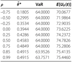
Table 1 Optimal investment strategies and expected results with different dependence parameters
ρ θ˜∗ VaR E[Uθ(t)]
–0.75 0.1805 64.0000 70.0677 –0.50 0.2995 64.0000 71.9864 –0.25 0.3534 64.0000 72.9035 0.00 0.3944 64.0000 73.6225 0.25 0.4286 64.0000 74.2372 0.50 0.4583 64.0000 74.7826 0.75 0.4849 64.0000 75.2806 0.85 0.4915 63.9526 75.4135 0.99 0.4915 63.7571 75.4460
interest rateδ= . and the log returns of some stock are modeled by
L(t) = .t+ .B(t) +
M(t)
i= ζi,
where{B(t),t≥}is a standard Brownian motion,M(t) is a homogeneous Poisson process with intensity , and the generic r.v.ζ followsN(–., .).
Assume without loss of generality that the investment period is [, ], and then we com-puteφ(–) = ., which is larger than the riskless interest rate. The numerical solution to the equationφθ() = isθ¯= .,i.e.the upper bound of the fraction invested in
risky asset.
Letx= be the initial capital andp= .%be the given probability, then the optimal strategies and expected results of investment with different dependence parameters are illustrated in Table .
From Table , it is easy to see that the fraction of risky investment increases as the de-pendence parameter goes up. The reason for this result is that the intensity and average rate of claims both decrease as the dependence parameter increases (see Proposition and Remark ). Thus the underwriting risks becomes smaller, more amount of wealth can be invested in risky asset. Meanwhile, the wealth at the end of the planning period gets more and the integrated risk equals the constraintC= when the fraction of risky investment are within the interval of investment strategies. In fact, the uniform asymptotic for the ruin probability also equals the upper bound .%. When the dependence parameter be-come so large that the optimal strategy exceeds the interval (,θ¯), the fraction of risky investmentθ˜∗is set toθ¯according to the convention, and the expected terminal wealth is still on the rise. Therefore, the connection between claim size and inter-arrival time has a direct impact on the optimal investment strategy and the expected result. The larger the dependence parameter is, the more favorable it is to the insurance company.
6 Conclusion
with some conditions more convenient to verify. Considering that the insurers may be more attentive to their future finite-time risks, the infinite-time discounted net loss in the definition of VaR which is considered by Kostadinova [] is replaced by a finite-time horizontal as the risk measure. Applying the asymptotic formula, an approximation of the optimal investment strategy depending on the dependence parameter and the time period is obtained and a numerical example is illustrated for the results. When investigating the impact of the dependence parameter, we find that the bigger the dependence parameter is, the more advantageous it is to the insurer. The reason for this result is explained by some inequalities.
Competing interests
The authors declare that they have no competing interests.
Authors’ contributions
All authors contributed equally to the manuscript read and approved the final manuscript.
Acknowledgements
The authors thank the referees for pointing out some errors in a previous version and for several comments that have led to improvement of this work. The research is supported by the National Natural Science Foundation of China
(NO. 11171221) and the Natural Science Foundation of Anhui Higher Education Institutions of China (NO. KJ2014B18).
Received: 12 November 2014 Accepted: 20 May 2015
References
1. Nikoloulopoulos, AK, Karlis, D: Fitting copulas to bivariate earthquake data: the seismic gap hypothesis revisited. Environmetrics19, 251-269 (2008)
2. Boudreault, M, Cossette, H, Landriault, D, Marceau, E: On a risk model with dependence between interclaim arrivals and claim sizes. Scand. Actuar. J.5, 265-285 (2006)
3. Albrecher, H, Teugels, J: Exponential behavior in the presence of dependence in risk theory. J. Appl. Probab.43, 265-285 (2006)
4. Cossette, H, Marceau, E, Marri, F: On the compound Poisson risk model with dependence based on a generalized Farilie-Gunmbel-Morgenstern copula. Insur. Math. Econ.43, 444-455 (2008)
5. Bargès, M, Cossette, H, Loisel, S, Marceau, E: On the moments of the aggregate discounted claims with dependence introduced by a FGM copula. ASTIN Bull.41, 215-238 (2011)
6. Asimit, AV, Badescu, AL: Extremes on the discounted aggregate claims in a time dependent risk model. Scand. Actuar. J.2, 93-104 (2010)
7. Yong, W, Xiang, H: Differential equations for ruin probability in a special risk model with FGM copula for the claim size and the inter-claim time. J. Inequal. Appl.2012, 156 (2012)
8. Yin, C, Wen, Y: An extension of Paulsen-Gjessing’s risk model with stochastic return on investments. Insur. Math. Econ. 52, 469-476 (2013)
9. Klüppelberg, C, Kostadinova, R: Integrated insurance risk models with exponential Lévy investment. Insur. Math. Econ.42, 560-577 (2008)
10. Heyde, CC, Wang, D: Finite-time ruin probability with an exponential Lévy process investment return and heavy-tailed claims. Insur. Math. Econ.41, 206-224 (2009)
11. Kostadinova, R: Optimal investment for insurers when the stock price follows an exponential Lévy process. Insur. Math. Econ.41, 250-263 (2007)
12. Asmussen, S, Albrecher, H: Ruin Probabilities. World Scientific, London (2010)
13. Emmer, S, Klüppelberg, C: Optimal portfolios when stock prices follow an exponential Lévy process. Finance Stoch.8, 17-44 (2004)
14. Cont, R, Tankov, P: Financial Modelling with Jump Processes. Chapman & Hall/CRC, Boca Raton (2004)
15. Li, J: Asymptotics in a time-dependent renewal risk model with stochastic return. J. Math. Anal. Appl.387, 1009-1023 (2012)
16. Fu, KA, Ng, CYA: Asymptotics for the ruin probability of a time-dependent renewal risk model with geometric Lévy process investment returns and dominatedly-varying-tailed claims. Insur. Math. Econ.56, 80-87 (2014)
17. Tang, Q, Wang, G, Yuen, KC: Uniform tail asymptotics for the stochastic present value of aggregate claims in the renewal risk model. Insur. Math. Econ.46, 362-370 (2010)