Linear convergence of the relaxed gradient projection algorithm for solving the split equality problems in Hilbert spaces

(1)

R E S E A R C H

Open Access

Linear convergence of the relaxed gradient

projection algorithm for solving the split

equality problems in Hilbert spaces

Tingting Tian

1

_{, Luoyi Shi}

1*

_{and Rudong Chen}

1

*_{Correspondence:} [email protected] 1_{Department of Mathematical}

Science, Tianjin Polytechnic University, Tianjin, P.R. China

Abstract

In this paper, we consider the relaxed gradient projection algorithm to solve the split equality problem in Hilbert spaces, and we investigate its linear convergence. In particular, we use the concept of the bounded linear regularity property for the split equality problem to prove the linear convergence property for the above algorithm. Furthermore, we conclude the linear convergence rate of the relaxed gradient projection algorithm. Finally, some numerical experiments are given to test the validity of our results.

Keywords: Linear convergence; Split equality problem; Bounded linear regularity; Relaxed gradient projection algorithm

1 Introduction

LetCandQbe nonempty closed convex subsets of real Hilbert spacesH1andH2, respec-tively, and letA:H1→H3andB:H2→H3be two bounded linear operators,H3is also a real Hilbert spaces. The split equality problem (SEP for short), as an important extension of the split feasibility problem, was first presented by Moudafi [1]. It can be mathematically characterized by finding pointsx∈Candy∈Qthat satisfy the property

Ax=By, (1.1)

which allows for asymmetric and partial relations between the variablesxandy.

The split equality problem has received plenty attention due to its extraordinary prac-ticality and wide applicability in many fields of applied mathematics; examples of such problems include decomposition methods for partial differential equations, applications in game theory and intensity-modulated radiation therapy (IMRT for short), for which comprehensive references are available [2,3]. In fact, various algorithms have been used in studies extensively to find a solution to the split equality problem. One of the most orig-inal and important algorithms is the alternating CQ algorithm (ACQA for short), which was proposed by Moudafi [1], and it has the following iterative form:

(ACQA)

⎧ ⎨ ⎩

xk+1=PC(xk–γkA∗(Axk–Byk)),

yk+1=PQ(yk+γkB∗(Axk+1–Byk)).

(1.2)

(2)

Then one proved the weak convergence of ACQA (1.2) provided that the solution set of SEP (1.1) is nonempty.

Since the ACQ algorithm involves two projectionsPCandPQ, it might be diﬃcult to cal-culate in the case where one of them does not have a closed-form expression. To solve this problem, Moudaﬁ [4] proposed the relaxed alternating CQ algorithm (RACQA for short) by using orthogonal projections onto half-spaces to replace the original closed convex sets, and it has the following iterative form:

(RACQA)

⎧ ⎨ ⎩

xk+1=PCk(xk–γA∗(Axk–Byk)),

yk+1=PQk(yk+βB ∗₍_Ax

k+1–Byk)).

(1.3)

Meanwhile, one proved that the above algorithm can converge weakly to a solution of SEP (1.1).

In the RACQA, the step size parameters do not vary. Then, as a quite important gen-eralization of the RACQA, Moudaﬁ [5] presented the relaxed simultaneous iterative al-gorithm (RSSEA for short), whose parameters are allowed to vary, and obtained a weak convergence result:

(RSSEA)

⎧ ⎨ ⎩

xk+1=PCk(xk–γkA∗(Axk–Byk)),

yk+1=PQk(yk+γkB ∗₍_Ax

k–Byk)).

Moreover, in order to obtain a strong convergence result, Shi et al. [6] improved Moudaﬁ’s algorithms and proposed the following algorithm:

⎧ ⎨ ⎩

xk+1=PC[(1 –αk)(xk–γkA∗(Axk–Byk))],

yk+1=PQ[(1 –αk)(yk+γkB∗(Axk–Byk))].

The above basic methods for solving the split equality problem are well known. For more information with regard to methods solving the split equality problem, see [7–9]. However, the convergence results of the above algorithms are not good enough and the convergence rate of these algorithms have not been explicitly estimated.

Recently, Shi et al. [10] presented the varying step size gradient projection algorithm for solving the SEP and obtained a linear convergence result. In particular, they conclude the linear convergent rate of the varying step size gradient projection algorithm. However, this algorithm is not easy to implement.

LetS=C×Q⊆H1×H2=:H,G= [A, –B] :H→H3, and the adjoint operator ofGis denoted byG∗. Then the problem (1.1) can be reformulated as to ﬁndw= (x,y)∈Swhich satisﬁesGw= 0. And then the relaxed simultaneous iterative algorithm (RSSEA) reduces to the following relaxed gradient projection algorithm (in short, RGPA):

(RGPA) wk+1=PSk

wk–γkG∗Gwk

.

(3)

linear convergence property for the CQ algorithm which is to solve the split feasibility problem, Wang et al. [11] presented the linear regularity property for the split feasibility problem. Motivated and inspired by their work, we devote our work to proving the linear convergence property for the RGPA with the bounded linear regularity property for SEP (1.1). For this purpose, we introduce the notion of the bounded linear regularity property for SEP (1.1), and use some suitable types of step sizes to prove the linear convergence property for the RGPA. In addition, we conclude the linear convergence rate of RGPA. Finally, some numerical experiments are given to test the validity of our results.

2 Preliminaries

For convenience, we introducing several notations. Throughout the whole paper, we as-sume thatHis a real Hilbert space whose inner product and norm are denoted by·,·and

· , respectively.Idenotes the identity operator onH. LetSbe a nonempty subset ofH, the relative interior ofSis denoted byriS.T∗is the adjoint operators ofT. We denote by

Band B the unit open ball and the unit closed ball with center at the origin, respectively, that is,

B:=v∈H:v< 1 and B:=v∈H:v ≤1.

There are several deﬁnitions and basic results that will be used in the proofs of our main results.

Deﬁnition 2.1([12]) A mappingT:H→Hgoes by the name of

(i) non-expansive, if

Tx–Ty ≤ x–y, ∀x,y∈H;

(ii) ﬁrmly non-expansive, if

Tx–Ty2≤ x–y,Tx–Ty, ∀x,y∈H.

For an elementw∈H and a setS⊂H, the distance ofwontoS and the orthogonal projection fromwontoS, denoted bydS(w) andPS(w), respectively, are deﬁned by

dS(w) =inf

v∈Sw–v and PS(w) =

v∈S:d(w,S) =w–v.

Some basic properties of an orthogonal projection were introduced by Bauschke et al. in [12], and they are listed in the following proposition.

Proposition 2.2([12]) Let S be a closed,convex,and nonempty subset of H,then,for any x,y∈H and z∈S,

(i) x–PSx,z–PSx ≤0;

(ii) PSx–PSy2≤ PSx–PSy,x–y;

(iii) PSx–z2≤ x–z2–PSx–x2.

(4)

Let G:H→H3 be a bounded linear operator. The kernel ofG is denoted kerG=

{y∈H:Gy= 0}, and the orthogonal complement ofkerGis denoted (kerG)⊥={x∈H:

y,x= 0,∀y∈kerG}. As is well known, bothkerGand (kerG)⊥are closed subspaces ofH. Throughout this paper, we useΓ to denote the solution set of SEP (1.1), that is,

Γ :={w∈S:Gw= 0}=S∩G–1(0) =S∩kerG.

We assume that the SEP is consistent, thus,Γ is a closed, convex, and nonempty set. Recall that a sequence{wk}inH is called linearly convergent to its limitw∗(with rate

α∈[0, 1)), if there existβ> 0 and a positive integerNsuch that

wk–w∗ ≤βαk for allk≥N.

To investigate the linear convergence property of the projection algorithm for solving convex feasibility problems, Zhao et al. [13] presented the linear regularity for a family of closed convex subsets in a real Hilbert space, as deﬁned below.

Deﬁnition 2.4([13]) Let{Si}i∈Ibe a family of closed convex subsets of a real Hilbert space

HandS=_i_∈_ISi= ∅. The family{Si}i∈Iis called bounded linearly regular if, for eacha> 0, there exists a constantγa> 0 such that

dS(w)≤γasup

dSi(w) :i∈I

for allw∈aB.

Bauschke [14] proved the following lemma for the caseHis the Euclidean space. It pro-vides suﬃcient conditions for the bounded linear regularity property for two closed con-vex subsets ofH.

Lemma 2.5([14]) Let E and F be closed convex subsets of H.Then E,F is bounded linearly regular provided that at least one of the following conditions holds:

(a) riE∩F=∅andFis a polyhedron;

(b) riE∩riF=∅andEis ﬁnite codimensional; (c) riE∩riF=∅andEis ﬁnite dimensional.

Next, we will introduce the concept of bounded linear regularity for SEP (1.1).

Deﬁnition 2.6([10]) SEP (1.1) is said to have the bounded linear regularity property if for eacha> 0, there exists a constantγa> 0 such that

γadΓ(w)≤ Gw for allw∈aB∩S. (2.1)

Shi et al. [10] construct some moderate suﬃcient conditions to ensure the bounded lin-ear regularity property for SEP (1.1). This is shown in the lemma below.

Lemma 2.7([10]) SEP(1.1)satisﬁes the bounded linear regularity property if one of the following conditions holds:

(5)

(c) riS∩kerG=∅andkerGis ﬁnite dimensional;

(d) riS∩kerG=∅,Ghas closed range andS=C×Qis ﬁnite codimensional; (e) riS∩kerG=∅,Ghas closed range andS=C×Qis ﬁnite dimensional.

Now, we will present the deﬁnition of sub-diﬀerential which is vital for constructing iterative algorithms later.

Definition 2.8([15]) Letf :H→Rbe a convex function. The sub-differential off atxis defined as

∂f(x) :=ξ∈H:f(y)≥f(x) +ξ,y–xfor ally∈H.

Lemma 2.9([15]) Let f :H→R be a convex function,x0∈H,and f be sub-diﬀerentiable

at x0.Suppose that D={x∈H:f(x)≤0}is nonempty for any g(x0)∈∂f(x0),deﬁneD by˜

˜

D:=x∈H:f(x0) +

g(x0),x–x0

≤0.

Then:

(i) D⊆ ˜D.Ifg(x0)= 0,thenD˜ is a half-space;otherwise,D˜ =H; (ii) PD˜(x0) =x0–max_g(x{f(x0),0}

0)2 g(x0); (iii) dD˜(x0) =

max{f(x0),0}

g(x0) .

Finally, in order to complete the convergence analysis, the following equality and con-cept of Fejér monotone sequence are essential.

Lemma 2.10([12]) Let{xi}i∈Ibe a ﬁnite family in H,and{λi}i∈Ibe a ﬁnite family in R with

i∈Iλi= 1,then the following equality holds:

i∈I

λixi

2=

i∈I

λixi2– 1 2

i∈I

j∈I

λiλjxi–xj2, i≥2.

Deﬁnition 2.11([12]) LetCbe a nonempty subset ofH, and{xi}be a sequence inH.

{xi}is called Fejér monotone with respect toC, if

xi+1–z ≤ xi–z, ∀z∈C.

Obviously,lim_i_→∞xi–zexists.

3 Main result

In this section, we mainly use the bounded linear regularity property for SEP (1.1) to prove the linear convergence of the relaxed gradient projection algorithm when using diﬀerent types of step sizes.

We start by reviewing the relaxed gradient projection algorithm in detail. Note that Moudaﬁ [5] presented the relaxed simultaneous iterative algorithm (RSSEA) for solving the approximate SEP and established its weak convergence:

(RSSEA)

⎧ ⎨ ⎩

xk+1=PCk(xk–γkA ∗₍_Ax

k–Byk)),

yk+1=PQk(yk+γkB∗(Axk–Byk)),

(6)

whereCkandQkare two sequences of closed convex sets, deﬁned by

Ck=

x∈H1:c(xk) +ξk,x–xk ≤0

, whereξk∈∂c(xk),

and

Qk=

y∈H2:q(yk) +ηk,y–yk ≤0

, whereηk∈∂q(yk),

wherec:H1→Randq:H2→Rare convex, sub-differentiable functions, and where the sub-differentials are bounded on bounded sets. Applying the definition of sub-differential, one finds thatC⊆CkandQ⊆Qk, whereCandQare two nonempty closed convex level sets:

C=x∈H1:c(x)≤0

,

and

Q=y∈H2:q(y)≤0

.

For convenience, we deﬁneh:H1×H2to be

h(w) =h(x,y) =c(x) +q(y),

then

C×Q⊆S, whereS=w∈H1×H2:h(w)≤0

.

We deﬁne

Sk=

w∈H1×H2:h(wk) +θk,w–wk ≤0

, whereθk∈∂h(wk),

then

S⊆Sk, Ck×Qk⊆Sk.

Moreover, letS=C×Q⊆H=H1×H2.G= [A, –B] :H→H3. The adjoint operator ofG is denoted byG∗. ThenGandG∗Ghave the following matrix form:

G= [A, –B], G∗G=

A∗A –A∗B

–B∗B B∗B

.

On that basis, the original problem (1.1) can be modiﬁed as

(7)

And then the algorithm (3.1) reduces to the following relaxed gradient projection algo-rithm (in short, RGPA):

(RGPA) wk+1=PSk

wk–γkG∗Gwk

. (3.3)

The lemma below will be a powerful tool in our proof later.

Lemma 3.1 Assume that a vector xk_{in S}

kminimizes the function f(t) =1₂Gt2over all t

in Sk.Then xk=PSk(x k_–_γ

k∇f(xk))withγk∈(0, +∞).

Proof Since a vectorxk_in_S

kminimizes the functionf(t) = 1₂Gt2over alltinSkwe have

∇f(xk_),_t_–_xk_≥_{0, where}_∇_f₍_xk_{) =}_G∗_Gxk_{. This is equivalent to}_xk_{– (}_xk_–_γ

k∇f(xk)),t–

xk_≥_{0 from which we infer that}_xk₌_P Sk(x

k_–_γ

k∇f(xk)). The proof is complete.

Now we give the main theorem and proof of this paper.

Theorem 3.2 Assume that SEP(3.2)satisﬁes the bounded linear regularity property.Then the sequence{wk}generated by RGPA(3.3)withγk∈(0, +∞)converges to a solution w∗of

SEP(1.1)such that

wk–w∗ ≤σp

k

i=1γi_, _(3.4)

forσ≥1and0 <p< 1,provided that one of the following conditions is assumed:

⎧ ⎪ ⎪ ⎪ ⎪ ⎪ ⎨ ⎪ ⎪ ⎪ ⎪ ⎪ ⎩

(a) 0 <lim_k_→∞infγk≤limk→∞supγk<_G22;

(b) γk=

⎧ ⎨ ⎩

0, wk∈Γ;

ρkGwk2

G∗Gwk2 and 0≤limk→∞infρk≤limk→∞supρk< 2, otherwise; (c) limk→∞γk= 0 and

∞

k=1γk=∞.

(3.5)

Consequently,{wk}converges to w∗linearly in the case when(a)or(b)is supposed.

Proof Without loss of generality, we assume thatwkis not inΓ for allk≥1. Otherwise, RGPA (3.3) terminates in ﬁnite number of iterates, and then the conclusions follow clearly. Firstly, we will show that the sequence{wk}is Fejér monotone with respect toΓ and the sequenceGwk2converges to zero.

Letz∈Γ, thenGz= 0, that is,zminimizesf(t) = 1₂Gt2_over_t_∈_S_{k, for all}_k_{. From} Lemma3.1,

z=PSkz=PSk

z–γkG∗Gz

, (3.6)

for allk. Since we have (3.6) andPSkis non-expansive, we obtain

z–wk+12

= PSk

z–γkG∗Gz

–PSk

(8)

≤ z–γkG∗Gz–wk+γkG∗Gwk 2

=z–wk2– 2γk

z–wk,G∗Gz–G∗Gwk

+γ_k2 G∗Gz–G∗Gwk 2

,

which is equivalent to

z–wk2–z–wk+12≥

2γk–γk2

G∗_Gw k2

Gwk2

Gwk2. (3.7)

Further, from the condition in (3.5), we get the following assertions:

(i) If (a) or (c) holds, then there existη> 0andM∈Nsuch that

γk≤η< 2

G2 for anyk≥M.

(ii) If (a) or (b) holds, then

lim

k→∞infγk> 0.

Using the above assertions, we deduce that there existsM∈Nsuch that

γ_k2 G∗Gwk ≤2Gwk, (3.8)

for anyk≥M, if (a), (b), (c) are assumed. Substituting (3.8) in (3.7), we see thatwk–zk≥M is monotone decreasing. From Deﬁnition2.11, we infer that the sequence{wk}is Fejér monotone with respect to Γ. Hencelim_k_→∞wk–zexists and the sequence Gwk2 converges to zero.

Then we show that the sequence{wk–wk+1}converges to zero. In view of the property of the orthogonal projection, we infer

wk+1–

wk–γkG∗Gwk

,z–wk+1

≥0,

that is,

wk–wk+1,z–wk+1 ≤γk

G∗Gwk,z–wk+1

≤γk G∗Gwk z–wk+1. (3.9)

Combining (3.9) and

wk–wk+12=z–wk2–z–wk+12+ 2wk+1–wk,wk+1–z,

we obtain

wk–wk+12≤ z–wk2–z–wk+12+ 2γk G∗Gwk z–wk+1.

Since the sequence{wk–z}is bounded, the right hand side converges to zero. Therefore, the sequence{wk–wk+1}converges to zero.

Next, we show that {wk} converges to a solutionw∗ of SEP and (3.4) holds. Because

wk+1∈Sk, we get

(9)

which implies that

h(wk)≤–θk,wk+1–wk ≤θwk+1–wk, whereθk ≤θfor allk.

Then there existsL∈N, whenk≥L, and by virtue of the sequence{wk–wk+1} converg-ing to zero, it follows thath(wk)≤0. Consequently,wk∈Sfor anyk≥L.

Since the SEP satisﬁes the bounded linear regularity property andwk∈Sfor allk≥L, there existsβ> 0 such that

βdΓ(wk)≤ Gwk, (3.10)

for allk≥L. Combining (3.10) with (3.7), we obtain

wk+1–z2≤ wk–z2–β2γk

2 –γk

G∗Gwk2

Gwk2

d2Γ(wk),

for eachz∈Γ, which equals

dΓ(wk+1)2≤

1 –β2γk

2 –γk

G∗_Gw k2

Gwk2

d2_Γ(wk). (3.11)

Note that if (a), (b) and (c) hold, then

lim

k→∞inf

2 –γk

G∗Gwk2

Gwk2

> 0.

Hence, there existsTsuch that

α=inf

k≥Tβ 2

2 –γk

G∗Gwk2

Gwk2

> 0. (3.12)

Using (3.12) and (3.11), we infer that

d_Γ2(wk+1)≤(1 –αγk)d2Γ(wk), for allk≥N=max{M,L,T}.

By induction,

dΓ2(wk+1)≤d2Γ(wN) k

i=N+1

(1 –αγi), (3.13)

for allk≥N=max{M,L,T}. Observe that, for eachz∈Γ,wk+1–zis monotone de-creasing fork, hence

wm–wk+1 ≤ wm–PΓ(wk+1) + wk+1–PΓ(wk+1)

≤2 wk+1–PΓ(wk+1) = 2dΓ(wk+1), (3.14)

for allm>k>N. Substituting (3.13) in (3.14), one can easily show that

wm–wk+1 ≤2dΓ(wN) k

i=N+1

(10)

for allm≥k+ 1. Letp:=e–α2 ∈_{(0, 1), then}

k

i=N+1

1 –αγi=exp

1 2

k

i=N+1

ln(1 –αγi)

≤pki=N+1γi_. _(3.16)

From (3.15) and (3.16), we get

wm–wk+1 ≤2dΓ(wN)p

k

i=N+1γi_, _{for all}_m≥_k_{+ 1.}

By virtue of∞_k=1γk=∞,{wk}is a Cauchy sequence and converges to a solutionw∗ of SEP (1.1) satisfying

wk+1–w∗ ≤2dΓ(wN)p

k

i=N+1γi_, _{for all}_k≥_N_.

For convenience, let

σ=max2dΓ(wN)p–

N

i=1γi_,_max _w

i–w∗ p–

i j=1γj

,i= 1, 2, . . . ,N. Then

wk–w∗ ≤σp

k i=1γi_.

Moreover, if (a) or (b) is assumed, thenlimk→∞infγk> 0. One can derive that{wk} con-verges tow∗linearly. This completes the proof.

As a direct consequence of Lemma2.7and Theorem3.2, we propose the following corol-lary.

Corollary 3.3 Assume that one of statements (a)–(e)of Lemma2.7holds. Then the se-quence{wk}generated by RGPA(3.3)withγk∈(0, +∞)converges to a solution w∗of SEP (3.2)satisfying(3.4),provided that one of the conditions in(3.5)is assumed.In particular,

{wk}converges to w∗linearly in the case when(a)or(b)in(3.5)is assumed.

4 Numerical experiments

In this section, we give an example to verify the validity of our results. All codes were writ-ten in Wolfram Mathematica (version 10.3). All the numerical procedures were performed on a personal Asus computer with AMD A9-9420 RADEON R5, 5 COMPUTE. CORES 2C+3G 3.00 GHz and RAM 8.00 GB.

LetH1=R,H2=R2andH3=R3. We have the SEP withC=Ck={x∈H2:x ≤20},

Q=Qk={x∈H1:X ≤10}, andA:H2→H3,B:H1→H3are deﬁned by

A(x,y) = (x,y, 0) and B(z) = (0,z, 0), for allx,y,z∈R,

respectively. LetS=C×Q⊆R3_{. Deﬁne an operator}_G_{= [}_A_{, –}_B_{] :}_S_→_H 3by

(11)

ThenkerG∩riS={(0,z,z),z∈Q} =∅,Sis ﬁnite codimensional,Ghas closed range, and the solution set of the SEP isΓ = (C×Q)∩kerG={(0,z,z) :z∈Q}. By Lemma2.7it is easy to show that the SEP satisﬁes the bounded linear regularity property.

Forw= (x,y,z)∈S, we have

dΓ2(w) =x2+ (y–z)2

2 .

Letw0= (x0,y0,z0)∈C×Q. In view of RGPA (3.3), we infer

⎧ ⎪ ⎪ ⎨ ⎪ ⎪ ⎩

xn+1=xn–γnxn,

yn+1= (1 –γn)yn+γnzn,

zn+1= (1 –γn)zn+γnyn.

In algorithm (3.3), we takeγn=1₂,_n+1n , respectively. Moreover, we select the error value to be 10–10_{, 10}–20_{, and initial value}_w

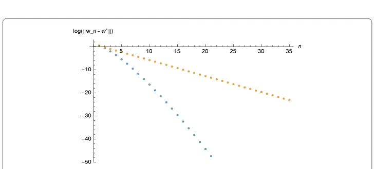
[image:11.595.118.477.351.497.2]

0= (3, 2, 8). Then we get the numerical results displayed in Figs.1and2.

Figure 1Thex-coordinate indicates the number of iterative steps and they-coordinate indicates the logarithm of the error. Initial conditions:x1= 3,y1= 2,z1= 8.w∗= (0, 5, 5), error = 10–10. :γn=1₂, :γn=_nn₊₁

[image:11.595.115.479.535.700.2]

(12)

Acknowledgements

The authors would like to express their sincere thanks to the editors and reviewers for their noteworthy comments, suggestions, and ideas, which helped to improve this paper.

Funding

This research was supported by NSFC Grants No:11226125;No:11301379;No:11671167.

Availability of data and materials

All data generated or analysed during this study are included in this published article.

Competing interests

The authors declare that they have no competing interests.

Authors’ contributions

The main idea of this paper was proposed by TT, LS and RC prepared the manuscript initially and performed all the steps of the proofs in this research. All authors read and approved the ﬁnal manuscript.

Publisher’s Note

Springer Nature remains neutral with regard to jurisdictional claims in published maps and institutional aﬃliations.

Received: 3 March 2019 Accepted: 15 March 2019

References

1. Moudaﬁ, A.: Alternating CQ-algorithm for convex feasibility and split ﬁxed-point problems. J. Nonlinear Convex Anal. 15(4), 809–818 (2013)

2. Censor, Y., Bortfeld, T., Martin, B.: A uniﬁed approach for inversion problems in intensity-modulated radiation therapy. Phys. Med. Biol.51, 2353–2365 (2006)

3. Censor, Y., Elfving, T., Kopf, N., Bortﬂed, T.: The multi-sets split feasibility problem and it applications to inverse problems. Inverse Probl.21, 2071–2084 (2005)

4. Moudaﬁ, A.: A relaxed alternating CQ-algorithms for convex feasibility problems. Nonlinear Anal., Theory Methods Appl.79, 117–121 (2004)

5. Byrne, C., Moudaﬁ, A.: Extensions of the CQ algorithm for split feasibility and split equality problems. hal-00776640-version 1 (2013)

6. Shi, L.Y., Chen, R.D., Wu, Y.J.: Strong convergence of iterative algorithms for split equality problem. J. Inequal. Appl. 2014, Article ID 478 (2014)

7. Zhao, Y., Shi, L.Y.: Strong convergence of an extragradient-type algorithm for the multiple-sets split equality problem. J. Inequal. Appl. (2017).https://doi.org/10.1186/s13660-017-1326-y

8. Dong, Q.L., He, S.N., Zhao, J.: Solving the split equality problem without prior knowledge of operator norms. Optimization64(9), 1887–1906 (2015)

9. Dong, Q.L., He, S.N.: Modiﬁed projection algorithms for solving the split equality problems. Sci. World J.2014, Article ID 328787 (2014)

10. Shi, L.Y., Ansari, Q.H., Wen, C.F.: Linear convergence of gradient projection algorithm for split equality problems. Optimization,67, 2347–2358 (2018)

11. Wang, J.H., Hu, Y.H., Li, C., Yao, J.C.: Linear convergence of CQ algorithms and applications in gene regulatory network inference. Inverse Probl.33, 055017 (2017)

12. Bauschke, H.H., Combettes, P.L.: Convex Analysis and Monotone Operator Theory in Hilbert Spaces. Springer, London (2011)

13. Zhao, X.P., Kung, F.N., Li, C.: Linear regularity and linear convergence of projection-based methods for solving convex feasibility problems. Appl. Math. Optim. (2017).https://doi.org/10.1007/s00245-017-9417-1

14. Bauschke, H.H.: Projection algorithms and monotone operators. Ph.D. thesis, Department of Math-ematics, Simon Fraser University, Burnaby, BC (1996)http://oldweb.cecm.sfu.ca/preprints/1996pp.html