Partial privatization and unidirectional transboundary pollution

Munich Personal RePEc Archive

Partial privatization and unidirectional

transboundary pollution

Kato, Kazuhiko

Faculty of Economics, Asia University

2 December 2010

Online at

https://mpra.ub.uni-muenchen.de/27155/

Partial privatization and unidirectional

transboundary pollution

†

Kazuhiko Kato

December 2, 2010

Abstract

We determine whether or not a local regional government should privatize its local public firm in a mixed duopoly when it faces the problem of unidirectional transboundary pollution. We consider two regions in an economy, one located upstream and the other, downstream. Where both the local public firm owned by the local government upstream and the private firm are located and compete upstream, we analyze two cases: (h) the private firm is owned by private investors upstream and (f) it is owned by private investors downstream. A comparison of the two cases presents the following results. Partial privatization is desirable for local welfare upstream in (h), but it is not always desirable in (f). In both (h) and (f), it is desirable for local welfare downstream and for the overall welfare of the economy when the degree of environmental damage and the fraction of transboundary pollution upstream are low. However, when they are high, the results change for (h) and (f).

JEL classification: L13; L33; Q53; R38

Keywords: Mixed Duopoly, Privatization, Transboundary pollution

†_{We thank the participants for their helpful comments in the non-linear economic theory workshop}

at Chuo University (November 2010).

‡_{Faculty of Economics, Asia University, 5-24-10 Sakai, Musashino shi, Tokyo 180-8629, Japan;}

1

Introduction

Transboundary pollution such as that caused by acid rain and water and air pollution

has been attracting attention since the middle-nineteenth century. For example, acid

rain, which has long been recognized as a serious environmental problem in Europe, has

become a serious issue in East Asia over the past few decades.1 _{For another example,}

for the past several years, waste that is believed to be generated in Russia, China, and

Korea has been regularly found on the shores of northern Japan, where it is carried by

the sea. To solve this problem, Japan and Korea held working-level talks in February

2009.

Meanwhile, global warming continues to worsen the environment worldwide. It can

affect the fraction of transboundary pollution to a large extent because global warming

may cause the Westerlies to meander and increase the frequency of natural calamities.2

Therefore, while analyzing the transboundary pollution problem, we pay attention to not

only the total amount of pollution but also its transboundary fraction from one region

to the other.

In some of the countries and regions mentioned above, there still exist mixed markets

where public and private firms compete. In these mixed markets, the privatization of

public firms is a major issue because it changes their objectives and thus, their behavior.

Since the welfare-maximizing public firm takes into consideration environmental

dam-age, the effect of privatization on social welfare depends on the affairs associated with

1

Nagase and Silva (2007) provide, in detail, the extent of damage caused by acid rain in China and

Japan. Ichikawa and Fujita (1995) estimate the contribution of China to be about one-half of the total

with respect to the wet deposition of sulfate in Japan. For other transboundary pollution issues, Ohara

et al. (2001) indicate the threat of an increase in ozone, sulfate, and nitrate, causative factors of the existing urban ozone in China, which may greatly impact the air quality in Japan in the future.

2

The meandering Westerlies will also affect the present amount of air-borne pollutants and toxic

chemicals (which cause acid rain) that are carried between the countries. Heavy rains transport city

waste that may be lying on the riverbed or in waste collection sites located along the river into the river.

Floods then transfer this waste to downstream areas. An increase in the atmospheric temperature and

surface level of the sea and a decrease in the salinity of the seas due to the melting glaciers may alter

transboundary pollution. In particular, when we consider the partial privatization of

public firms, the welfare-maximizing degree of this partial privatization may be affected

by the fraction of transboundary pollution. Of course, in many cases, partial

privatiza-tion in one country or region affects not only its own welfare but also welfare of other

countries or regions through changes in the equilibrium outcome, including the influence

of transboundary pollution. We therefore pose the following two questions: (1) How does

the fraction of transboundary pollution affect the welfare-maximizing degree of partial

privatization? (2) Does partial privatization in one country or region enhance welfare of

other countries or regions and that of the whole world?

In order to answer these questions, we have developed a model. The model considers

two regions, with one located downstream of the other, and two firms, a public firm

and a private firm. In our model, the market is opened only upstream, and both firms

exist there. We consider two cases: (h) the private firm is owned by private investors

upstream and (f) it is owned by private investors downstream. In the literature of the

mixed oligopoly theory, we often observe different results between (h) and (f).3 _This

is because the behavior of the public firm changes from (h) to (f) and the profit of the

private firm is included in the objective of the public firm in (h) but not in (f).

In recent years, some studies have addressed the environmental issue in a mixed

oligopoly. B´arcena-Ruiz and Garz´on (2006), Beladi and Chao (2006), Wang and Wang

(2009), and Wang, Wang, and Zhao (2009) consider emission tax in the domestic

mar-ket, whereas Ohori (2006a, 2006b) considers the same in the international market. Kato

(2006, 2010) and Naito and Ogawa (2009) compare some environmental policies. They

examine environmental regulation in a mixed oligopoly and analyze the effects of

priva-tization. Cato (2008) investigates the relationship between the degree of environmental

damage and privatization. However, because these works deal with the environmental

problem in one region, they do not take into consideration transboundary pollution.

From among the earlier work conducted on transboundary pollution, Nagase and

3

For example, Fjell and Pal (1996), Fjell and Heywood (2004), Matsumura (2003), and Lu (2006)

demonstrate the different results in the case wherein the competitors of the public firm are domestic

Silva (2007) is closely related to our motivation. Nagase and Silva (2007) consider the

situation where one region (China) is located upstream of another region (Japan) under

unidirectional transboundary pollution.4 _{However, their main interest is to examine an}

environmental policy-making game between the two, and therefore, it differs from ours

with regard to focusing on the effect of privatization. In China, a large number of public

firms have been privatized since the 1990s.5 _{However, mixed oligopoly is still prevalent}

in several industries that depend on energy from fossil fuels, especially coal. Thus, the

analysis of transboundary pollution in the framework of the mixed oligopoly theory may

lead to a new approach in the research on the transboundary pollution problem.

The remainder of the paper is organized as follows. Section 2 describes our model.

Section 3 derives the equilibrium outcome under different cases of private firm ownership

and conducts a welfare comparison. Section 4 compares the results obtained in the

previ-ous section. Section 5 concludes the main text. Detailed calculations for the equilibrium

outcome in each case and proofs of the propositions are given in the Appendices.

2

Model

Consider an economy of two regions: regions A and B. Region A is located upstream

of region B. In this economy, there is one local public firm (firm 0) owned by the local

regional government of A and one private firm (firm 1) owned by private investors from

either region A or region B. Both the firms are located in region A and produce a

homogeneous product that harms the environment. We call this product a “dirty good.”

Firms 0 and 1 compete in quantity. The output of firm i is denoted by qi (i= 0,1).

Total output is denoted by Q = q0+q1. We assume that the cost function of firm i is

given by ci(qi) =cq2i/2. Given the inverse demand function of the dirty good, p=p(Q),

4

Nagase and Silva (2007) consider a competitive market and allow an abatement effort and an

emission tax policy.

5

For an overview of the reform of state-owned enterprises in China, see Fern´andez and Fern´

and then, the profit of firm i is

πi(q0, q1) = p(Q)qi−

ciqi

2 .

A representative consumer exists in each region. The representative consumer in

region A consumes the dirty good and a clean numeraire good. The representative

consumer in region B only exists.

The representative consumer in regionAmaximizesU(Q) +ysubject topQ+y =m,

where p denotes the price of the dirty good, y denotes the amount of the numeraire

good, whose price is normalized to 1, and m denotes the income of the representative

consumer. We assume that U(Q) is

U(Q) = aQ₋Q 2

2 . (1)

Therefore, we obtain the following inverse demand function,p(Q) =a₋Q by solving

the utility maximization problem of the representative consumer in regionA.

In our model, pollution is generated by either production or consumption and is

harmful to the environment. Producing or consuming one unit of a dirty good

gener-ates one unit of pollution. The pollution is converted into environmental damage which

reduces the consumer surplus via a lump-sum transfer. We do not consider the case

where pollution is generated by both production and consumption. In our setting,

pol-lution is generated only in regionA and there is no difference between pollution through

production and that through consumption. Therefore, in the subsequent instructions

and analyses, we consider the case that pollution is generated by production. The total

pollution in region l is denoted by El (l = A, B); the total environmental damage in

region l is denoted by Dl(El) = d(El)2/2.

We assume that pollution is transboundary and can affect the environment in region

B. We now explain how transboundary pollution is considered in the model. Pollution

is generated only in region A because both firms produce in region A; the amount of

pollution generated is Q. We assume that region A is located upstream of region B

(along a river or in the path of a periodic wind), and therefore, some of the pollution is

therefore, the fraction of pollution transported to regionB is (1₋θ). Thus, the pollution

levels in regions A and B are θQand (1₋θ)Q, respectively.

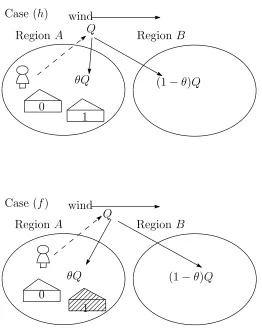
This paper examines two cases of ownership of the private firm: case (h), where firm

1 is owned by private investors from regionA, and case (f), where it is owned by private

investors from region B. Figure 1 shows the two cases and the amount of pollution of

two regions by the unidirectional transboundary pollution.

In the model, welfare is defined as the sum of consumer surplus, producer surplus,

and environmental damage.

First, we consider case (h), wherein firm 1 is owned by private investors from region

A. Welfare in region A is given by

wA= ∫ Q

0

p(s)ds₋ cq 2 0 2 − cq2 1 2 − d(θQ)2

2 +m. (2)

Welfare in region B is given by

wB =−

d_{(1₋θ)Q_}2

2 . (3)

Welfare in the economy is defined as the sum of the welfare in regions A and B. Thus,

W =

∫ Q

0

p(s)ds₋cq 2 0 2 − cq2 1 2 − d(θQ)2 2 −

d_{(1₋θ)Q_}2

2 +m. (4)

Second, we consider case (f). In this case, firm 1 is owned by private investors from

regionB. Welfare in regionA, welfare in regionB, and the total welfare are respectively

given by

wA = ∫ Q

0

p(s)ds₋p(Q)q1− cq2

0 2 −

d(θQ)2

2 +m, (5)

wB = p(Q)q1−

cq2 1 2 −

d_{(1₋θ)Q_}2

2 , (6)

W =

∫ Q

0

p(s)ds₋ cq 2 0 2 − cq2 1 2 − d(θQ)2 2 −

d_{(1₋θ)Q_}2

2 +m. (7)

We denote the welfare of region l as “local welfare l” and the welfare in the entire

economy as “total welfare.” Further, we define the local regional government oflas “local

Here, we define the objective function of each firm. The objective functions of public

firm U0 and private firm U1 are respectively given by

U0 = αW + (1₋α)π0, α _∈[0,1], (8)

U1 = π1. (9)

When α = 0, firm 0 is a pure profit-maximizer, and when α = 1, it is a pure local

welfare-maximizer. Here, α is understood as the share holding of the public sector and

1₋αis that of the private sector.6 _{The objective of firm 1 is to maximize its own profits.}

Finally, we consider the following timing of the game. Before the game begins, the

public firm is perfectly owned by local government A, that is, α = 1. When the game

starts, local government A chooses the level of α, and then, the two firms choose their

quantity simultaneously.

3

Equilibrium outcomes and welfare comparison

In this section, we derive the equilibrium outcome and compare three types of welfare

before and after privatization in cases (h) and (f). First, we examine case (h).

3.1

Case (

h

)

We first consider the case where firm 1 is owned by private investors from region A.

Local welfare A, local welfare B, and total welfare are respectively defined as (2),

(3), and (4).

In the second stage, each firm maximizes its objective by choosing its quantity. The

first-order condition of the maximization problem of firms 0 and 1 are respectively given

by

∂U0

∂q0 =a−(2−α+c+dαθ 2_)q0

−(1 +dαθ2)q1 = 0, (10) ∂U1

∂q1 =a−q0−(2 +c)q1 = 0. (11)

6

Solving the above first-order conditions, we obtain

qh

0 =

a(1 +c₋dαθ2₎

(1 +c)(3 +c)₋(2 +c)α+ (1 +c)dαθ2, (12)

qh

1 =

a(1 +c₋α+dαθ2₎

(1 +c)(3 +c)₋(2 +c)α+ (1 +c)dαθ2, (13)

whA=

2a2_{(1 +c){(1 +c)(4 +c−2dθ}2_{)−(5 + 2c−4dθ}2_−2cdθ2_)α} 2_{(1 +c)(3 +c)₋(2 +c)α+ (1 +c)dαθ2_}2 ,

+ a

2_α2

{3 +c₋dθ2(3 + 2cdθ2)_}

2_{(1 +c)(3 +c)₋(2 +c)α+ (1 +c)dαθ2_}2, (14)

wBh = −

a2_{d(2 + 2c−α)}2_(1−θ)2

2_{(1 +c)(3 +c)₋(2 +c)α+ (1 +c)dαθ2_}2, (15)

Wh = a

2_{{2(1 +c)}2_{(4 +c−2d)−2(1 +c)(5 + 2c−2d)α−2dα}2_θ2_{(2 +cdθ}2_)} 2_{(1 +c)(3 +c)₋(2 +c)α+ (1 +c)dαθ2_}2

+a

2_{{(3 +c−d)α}2_{+ 2d(2 + 2c−α)}2_{θ+ 4d(1 +c)(−2−2c+ 3α+cα)θ}2_} 2_{(1 +c)(3 +c)₋(2 +c)α+ (1 +c)dαθ2_}2 +m,

(16)

where the superscript h denotes the equilibrium outcome in the second stage in case

(h) except for α. With regard to α, the superscript denotes the equilibrium outcome

in the full game. In the subsequent section, this superscript is also used to represent

the equilibrium outcome in the second stage. To restrict our attention to the case of

the interior solution, we assume that 1 +c_≥ d. We also assume that c_≥ 1 in order to

simplify the subsequent analyses.

Here, we examine the comparative statics for the equilibrium output of each firm

with respect to α. We find that

∂qh

0 ∂α <0,

∂qh

1

∂α >0, and ∂Qh

∂α <0, if and only if dθ 2 _> 1

2. (17)

In terms of local welfare A, there are two distortions in the region. One is caused by

underproduction with regard to the duopolistic market and the other is caused by excess

production with regard to environmental damage. A high level of d and θ imply that a

large fraction of pollution remains in region A and environmental damage is large. In

this case, the latter distortion dominates the former one, and therefore, the local public

firm decreases its output when it gives greater weight to local welfareA.

A.7 _{Solving for α, we obtain}

αh = (1 +c) 2

1 + 3c+c2. (18)

The result shows that partial privatization is desirable for local welfare A. We also find

that αh _{does not depend on the fraction of transboundary pollution and the degree of}

environmental damage. Rather, these results depend on the functional forms of demand,

cost, and environmental damage.8

Does partial privatization of the local public firm enhance local welfare in

the other region and the total welfare? (welfare comparison)

We examine whether the optimal privatization for local welfare A enhances local

welfare B and the total welfare. Comparing local welfare B and total welfare at α = 1

and α=αh_{, we obtain the following proposition.}

Proposition 1. When θ = 1 or dθ2 _{= 1/2, w}

B|α=1 =wB|α=αh. Consider the case where θ _̸= 1 and dθ2 _{̸= 1/2. Then,}

wB|α=1−wB|α=αh >0 if d > 1

2 and θ ∈

(√

1 2d,1

)

,

wB|α=1−wB|α=αh <0 if







d > 1

2 and θ∈

[

0,√1 2d

)

,

d < 1₂ and θ_∈[0,1).

Proof. See Appendix B.

Figure 2 illustrates Proposition 1 for each value of the fraction of transboundary

pollution and the degree of environmental damage.

The intuition behind Proposition 1 is as follows. When θ = 1, no fraction of the

pollution caused in regionA is transported to regionB, and therefore,α does not affect

7

The second-order condition of the maximization problem is satisfied. See Appendix A.

8

The amount of total output and output level of each firm affect the decision with respect to αh.

Specifically, the total output level affects both the marginal utility of the representative consumer and the

marginal environmental damage. The larger is the total output, the larger are the marginal utility and

marginal environmental damage. On the other hand, the output level of each firm affects its marginal

production cost: the difference between the marginal production costs of firms is maximized at α= 1

and minimized atα= 0. As local government choosesαtaking into account both total output level and

local welfare B. When θ _̸= 1, some portion of the pollution generated in region A is

transported to region B. Local welfare B is based on environmental damage. We know

that the environmental damage function is a function of the total output and that the

total output decreases (increases) with an increase in α when θ > (_≤) 1/√2d. Suppose

the case where d and θ are small (large). When the local public firm is not privatized,

that is,α = 1, it produces more (less) and the total output is larger (smaller) than when

α=αh_{. The larger (smaller) the total output is, the larger (smaller) the total emission}

is. Therefore,α =αh _{(α= 1) is more desirable than α= 1 (α=α}h_{) for local welfareB.}

Next, we investigate the total welfare. We compare total welfare atα= 1 andα =αh_.

Calculating W_|α=1−Wα=αh, we obtain the following proposition.

Proposition 2.

W_|α=1−W|α=αh >0 if d > 1

2 and θ ∈

(√

1 2d,θ¯

]

,

W_|α=1−W|α=αh <0 if



   

   

d > 1₂ and θ _∈[0,√₂1_d),

d > 1

2 and θ ∈[¯θ,1], d < 1₂ and θ _∈[0,1],

where ¯θ is the solution of W_|α=1−Wα=αh = 0.

Proof. See Appendix C.

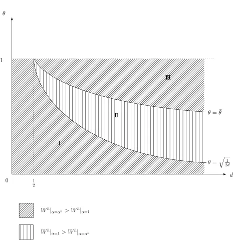
The intuition behind Proposition 2 is as follows. When θ and d are small, we find

that partial privatization enhances welfare of both regions A and B from (18) and

Propo-sition 1. Therefore, the total welfare is larger after partial privatization. When θ and

d are large, partial privatization increases local welfareA but decreases local welfare B.

Remember that local welfare B is composed of ₋DB(EB) and EB = (1−θ)Qh. When

θ and d are sufficiently large, EB becomes sufficiently small. A decrease of local welfare

B is overcome by an increase of local welfare A. Therefore, the total welfare is larger

under partial privatization when θ and d are either small or large. Figure 3 shows these

3.2

Case (

f

)

We consider the case where firm 1 is owned by private investors from region B.

Local welfare A, local welfare B, and total welfare are respectively defined as (5),

(6), and (7).

In the second stage, each firm maximizes its objective by choosing its quantity. The

first-order condition of the maximization problem of firms 0 and 1 are respectively given

by

∂U0

∂q0 = a−(2−α+c+dαθ 2_)q0

−(1₋α+dαθ2)q1 = 0, (19) ∂U1

∂q1 = a−q0−(2 +c)q1 = 0. (20)

Solving the above first-order conditions, we obtain

q₀f = a(1 +c+α−dαθ 2₎

(1 +c)(3₋α+c+dαθ2₎, (21)

q₁f = a(1 +c−α+dαθ 2₎

(1 +c)(3₋α+c+dαθ2₎, (22)

wf_A= a

2_{{(1 +c)}2_{(6 +c−4dθ}2_{)−2(1 +c)cα(1−dθ}2_{)−(2 + 3c)(1−dθ}2₎2_α2_}

2(1 +c)2_{(3−α+c+dαθ}2₎2 , (23)

wf_B = a

2_{{(2 +c)(1 +c−α)}2_{−4(1 +c)}2_{(1−2θ)d+ (2 +c)α}2_dθ4_} 2(1 +c)2_{(3−α+c+dαθ}2₎2

+ 2a

2_{(−2−4c−2c}2_{+ 2α+ 3cα+c}2_α−2α2 _−cα2_)dθ2

2(1 +c)2_{(3−α+c+dαθ}2₎2 , (24)

Wf = a

2_{{(1 +c)}2_{(4 +c−2d−2α+ 4dθ−4dθ}2_{+ 2dαθ}2_)−cα2_(1−dθ2₎2_}

(1 +c)2_{(3−α+c+dαθ}2₎2 +m. (25)

Here, we analyze the comparative statics for the equilibrium output of each firm with

respect to α. We find that

∂q₀f ∂α <0,

∂qf₁

∂α >0, and ∂Qf

∂α <0, if and only if dθ

2 _{>1. (26)}

In the first stage, local government A chooses α in order to maximize local welfare

A. Solving for α, we obtain9

9

In Appendix D, we show that the second-order condition of the maximization problem is satisfied.

αf =                                      ¯ α if           

0< d < c

1+2c and θ∈[0,1], c

1+2c < d and θ ∈[0,

√ _c

d(1+2c)], 3+2c

2(1+c) < d and θ ∈[

√

3+2c

2d(1+c),1],

1 if      c

1+2c < d <1 and θ∈[

√ _c

d(1+2c),1], 1< d and θ _∈[√ c

d(1+2c),

√ 1 d], 0 if   

1< d < 3+2c

2(1+c) and θ∈[

√

1

d,1],

3+2c

2(1+c) < d and θ∈[

√

1

d, √

3+2c

2d(1+c)], where

¯

α= (1 +c){3 + 2c−2dθ

2_{(1 +c)}}

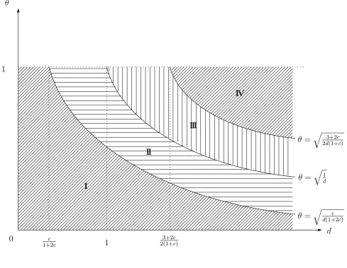
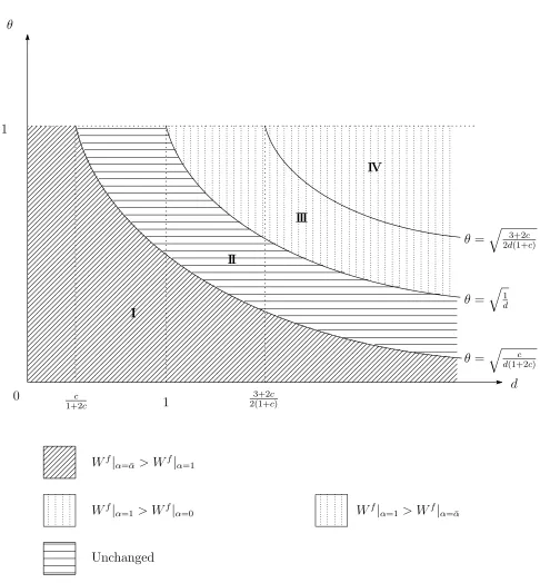
(3 + 6c+ 2c2_)(1−dθ2₎ . (27) From the result, we find that αf _{depends on the fraction of transboundary pollution}

and the degree of environmental damage. Figure 4 illustratesαf _{for eachdandθ. When}

bothdandθ are small or large (regionI orIV), partial privatization (αf _{= ¯α) is chosen.}

When they take a middle value, local public firm A is fully privatized (regionIII) or is

not privatized at all (region II).

The intuition behind the result is as follows. First, we consider the case where d

and θ are sufficiently large. In this case, environmental damage is severe in region A,

and thus, the local public firm produces less when α = 1 than when α = ¯α. Suppose

a marginal decrease of α at α = 1. A marginal increase of output of the public firm

does not affect welfare because the public firm is a local welfare maximizer when α= 1.

However, the marginal decrease of output of the private firm improves welfare because

it reduces the environmental damage. Therefore, partial privatization enhances welfare.

Second, we consider the case where d and θ are sufficiently small. In this case, the

degree of environmental damage is low, and thus, we regard this case as no environmental

problem in a mixed duopoly to some extent. Suppose a marginal decrease ofαatα= 1.

As is the same reason mentioned in the previous paragraph, a marginal decrease of

output of the public firm does not affect welfare. However, a marginal increase of output

of the private firm increases consumer surplus. Therefore, partial privatization enhances

Finally, we consider the case where d and θ take a middle value. In this case, the

equilibrium output in a mixed duopoly is nearly the same as that in a pure duopoly. For

example, consider the case wheredθ2 _{= 1. In this case, the reaction function of the local}

public firm does not depend on α: the reaction function of each firm is symmetric. And

thus, either full privatization or no privatization can be chosen.

Does privatization of the local public firm enhance local welfare in the

other region and the total welfare? (welfare comparison)

We examine whether the optimal privatization for local welfare A enhances local

welfareB and the total welfare. We compare local welfare B and total welfare at α= 1

and α=αf_.

Here, we compare local welfare B before and after privatization. Because the level

of αf _{depends on the values of parameters, we separate the cases for each α}f_{. Figure 4}

shows the level of αf _{for the values of parameters: ¯α is chosen by the local government}

A in regions I and IV, 0 in region III, and 1 in region II. In each region, the results of

the welfare comparison before and after privatization are as follows.

Proposition 3.

wB|α=1−wB|α= ¯α >0 if d > ₂₍₁₊3+2c_c) and θ ∈ (√

3+2c

2d(1+c),1

]

,

wB|α=1−wB|α= ¯α <0 if 

 

 

d > c

1+2c and θ ∈ [

0,√ c d(1+2c)

)

,

d < c

1+2c and θ ∈[0,1]

wB|α=1−wB|α=0 >0 if d >1 and θ ∈

(√

1

d, √

3+2c

2d(1+c)

]

.

Proof. See Appendix F.

According to Proposition 3, when the degree of environmental damage and the

frac-tion of transboundary pollufrac-tion remaining in regionA are low, privatization of the local

public firm in region A enhances local welfare B, but when they are high, privatization

worsens the welfare. Figure 5 shows these results.

The intuition behind Proposition 3 is as follows. Local welfareB is based on the sum

of firm 1’s profit and environmental damage. We know that the environmental damage

increase inα whenθ >1/√d. We also see that firm 1’s profit increases with an increase

inα whenθ >1/√dbecause the price of the dirty good increases with an decrease in the

total output, and the output of firm 1 increases as a result of the strategic substitution

effect. Thus, we find that local welfare B increases with an increase in α when θ >

1/√d. Whenθ < 1/√d, the results are opposite, that is, local welfareB decreases with

an increase in α.

Lastly, we compare total welfare between α = 1 and α = αf_{. As in the case of the}

welfare comparison for region B, we separate the cases for each αf_{. The results of the}

welfare comparison in terms of before and after privatization are as follows for each case.

Proposition 4.

W_|α=1−W|α= ¯α >0 if d > ₂₍₁₊3+2c_c) and θ∈ (√

3+2c

2d(1+c),1

]

,

W_|α=1−W|α= ¯α <0 if 

 

 

d > ₁₊₂c _c and θ _∈

[

0,√_d(1+2c _c)

)

,

d < c

1+2c and θ ∈[0,1]

W_|α=1−W|α=0 >0 if d >1 and θ ∈

(√

1

d, √

3+2c

2d(1+c)

]

.

Proof. See Appendix G.

Figure 6 shows Proposition 4. According to Proposition 4, when the degree of

en-vironmental damage and the fraction of transboundary pollution remaining in region

A are low, privatization of the local public firm in region A enhances the total welfare

because local welfare A and B both increase. However, when the same are high, local

welfare B is worsened considerably, and the total welfare decreases. Thus, in terms of

total welfare, privatization is not desirable.

4

Comparison between cases (

h

) and (

f

)

We compare the results obtained in cases (h) and (f). There are three major points.

1. Partial privatization is chosen in case (h), but partial privatization, full

2. Partial privatization enhances wA, wB, and W in both cases when the degree of

environmental damage and the fraction of transboundary pollution remaining in

region A are low.

3. Partial privatization enhances W and reduces wB in case (h), but it reduces both

wB and W in case (f) when the degree of environmental damage and the fraction

of transboundary pollution remaining in region A are high.

5

Concluding remarks

This paper examines the effect that the privatization of a local public firm has on local

welfare in two regions and on the overall welfare of the two regions when the fraction of

unidirectional transboundary pollution varies. We analyze this problem by considering

two separate cases of ownership of a private firm.

We discuss the possible implication of our results. Consider the example of the

rela-tionship between China upstream and Japan downstream. Since the twenty-first century,

several Japanese firms have entered the Chinese market. From China’s point of view,

it is more complex to calculate the optimal degree of privatization in terms of welfare

of China in this situation than in the situation where the competitor of the public firm

is a domestic private firm; the optimal degree of privatization varies for each value of

the degree of environmental damage and the fraction of transboundary pollution. When

the pollutant has a moderate degree of environmental damage, the Chinese government

should pay particular attention to the trend of the fraction of transboundary pollution,

since there is a possibility that its fraction is affected by recent extreme weather

condi-tions.

This paper uses a simple framework to consider the privatization problem in the

context of the unidirectional transboundary pollution problem. Therefore, several

ex-tensions of this analysis are possible. For example, we can consider the case wherein

firms can abate the possible pollution. If firms can reduce their pollution by investing

some abatement effort, the public firm produces more when it can invest abatement

to reduce pollution. As a result, the welfare-maximizing degree of partial privatization

changes and the effect of partial privatization of the upstream public firm on welfare of

each region might change to a large extent. We can also extend our model to examine

the case wherein a market for dirty goods exists in both countries, wherein a generation

of pollution occurs in the country located downstream, and wherein the government can

impose the environmental regulations such as emission taxes and quotas on firms. We

leave these analyses for future research.

Appendix A

The first-order condition of the maximization problem of local government

APartially differentiating wh

A with respect toα, we obtain

∂wh A

∂α =

a2_{(1 +c){(1 +c)}2_{−(1 + 3c+c}2_{)α}(1−2dθ}2₎2

{(1 +c)(3 +c+dαθ2_{)−(2 +c)α}}2 = 0. (28) We can easily find that the denominator is positive. We focus on the numerator.

When dθ2 _{= 1/2,w}h

A does not depend onα. When dθ2 ̸= 1/2, we can derive the optimal

degree of partial privatization level for local government A, that is, αh_.

The second-order condition of the maximization problem of local

govern-ment A

To determine whether αh _{is the maximizing value for w}h

A, we calculate the

second-order condition of the maximization problem for local government A. Then, we obtain

∂2_wh A

∂α2 =−

a2_{(1 +c)(1−2dθ}2₎2_{X0(c, d, θ, α)}

{(1 +c)(3 +c+dαθ2_{)−(2 +c)α}}4 ≤0, (29) where

X0(c, d, θ, α) = (1 +c)(₋3 +c+ 3c2+c3) + 2(2 +c)(1 + 3c+c2)α

+(3₋2α)dθ2+ (9₋8α)cdθ2+ (9₋8α)c2dθ2

+(3₋2α)c3dθ2 >0. (30)

Note that a strict inequality holds whendθ2 _{̸= 1/2. Therefore, the second-order condition}

Appendix B

Proof of Proposition 1. Calculating local welfare B when α= 1 andα =αh_{, we}

respec-tively obtain

wh

B|α=1 = −

a2_{(1 + 2c)}2_(1−θ)2_d

2_{1 + 3c+c2_{+ (1 +c)dθ}2_}2, (31)

wh

B|α=αh = −

a2_{(1 + 5c+ 2c}2₎2_(1−θ)2_d

2_{1 + 7c+ 5c2_+c3_{+ (1 +c)}2_dθ2_}2. (32)

Comparing the above, we obtain the following equation:

wh

B|α=1−whB|α=αh =

−a

2_{cd(1 +c)(1−θ)}2_(1−2dθ2_{){2 + 17c+ 37c}2_{+ 22c}3 _{+ 4c}4_{+ 2(1 +c)(1 + 4c+ 2c}2_)dθ2_} 2_{1 + 3c+c2_{+ (1 +c)dθ}2_}2_{{1 + 7c+ 5c}2_+c3_{+ (1 +c)}2_dθ2_}2 .

From the above equation, we find that wB|α=1 = wB|α=αh when θ = 1. Consider the

case where θ _̸= 1. Whether or notwB|α=1−wB|α=αh is positive depends on the sign of

1₋2dθ2. Thus, we can derive Proposition 1.

Appendix C

Proof of Proposition 2. Calculating the total welfare when α = 1 and α = αh_{, we}

re-spectively obtain

Wh

|α=1 =

a2_{{1 + 5c+ 8c}2_{+ 2c}3_{+ (1 + 2c)}2_{(2θ−1)d−4c}2_dθ2_−2cd2_θ4_} 2(1 + 3c+c2_+dθ2_+cdθ2₎2 +m,

(33)

Wh

|α=αh =

a2_{{(1 + 6c+ 2c}2_{)(1 + 7c+ 5c}2_+c3_{) + (1 + 5c+ 2c}2₎2_(2θ−1)d} 2(1 + 7c+ 5c2_+c3_+dθ2_{+ 2cdθ}2_+c2_dθ2₎2

−a

2_{{4c(1 + 7c+ 5c}2_+c3_)dθ2_{+ 2c(1 +c)}2_d2_θ4_}

2(1 + 7c+ 5c2_+c3_+dθ2_{+ 2cdθ}2_+c2_dθ2₎2 +m. (34)

The difference between them is

Wh_|α=1−Wh|α=αh =

a2_{c(−1 + 2dθ}2_{)X1(c, d, θ)}

where

X1(c, d, θ) =c+ 7c2+ 5c3+c4+ 2d+ 19cd+ 54c2d+ 59c3d+ 26c4d+ 4c5d

−2(1 +c)(2 + 17c+ 37c2 _{+ 22c}3_{+ 4c}4_)dθ

+ 2d(1 + 9c+ 21c2_{+ 25c}3_{+ 12c}4_{+ 2c}5_{+d+ 6cd+ 11c}2_{d+ 8c}3_{d+ 2c}4_d)θ2

−4(1 +c)2_{(1 + 4c+ 2c}2_)d2_θ3_{+ 2(1 +c)}3_{(1 + 2c)d}2_θ4_{. (35)}

When dθ2 _{= 1/2, there is no difference between them. We consider the case where}

dθ2 _{̸= 1/2. Whether or not the difference is positive depends on both the sign of−1+2dθ}2

and that ofX1(c, d, θ). At first glance, it is not clear whether or notX1(c, d, θ) is positive.

In the subsequent analyses, we examine the property of X1(c, d, θ).

First, we check the monotonicity of X1(c, d, θ) in θ _∈ [0,1]. Partially differentiating

X1(c, d, θ) with respect to θ, we find that

∂X1(c, d, θ)

∂θ =2d{−(1 +c)(2 + 17c+ 37c

2_{+ 22c}3 _{+ 4c}4₎

+ 2(1 + 9c+ 21c2+ 25c3+ 12c4 + 2c5+d+ 6cd+ 11c2d+ 8c3d+ 2c4d)θ

−6(1 +c)2(1 + 4c+ 2c2)dθ2+ 4(1 +c)3(1 + 2c)dθ3_}. (36)

Summing up the above terms, we find that ∂X1(c, d, θ)/∂θ= 2dX2(c, d, θ), where

X2(c, d, θ) =₋2(1₋θ)_{1 + 9c+ 21c2+ 25c3+ 12c4+ 2c5+ 2(1 +c)3(1 + 2c)dθ2_}

+ 2(1₋θ)(1 +c)2_{(1 + 4c+ 2c}2_{)dθ−c(1 + 12c+ 9c}2_{+ 2c}3₎

−4c(1 +c)2_dθ2_{. (37)}

The above calculation shows that the second term is positive whereas the other terms

are negative. As the upper bound ofd is assumed to be 1 +c, we substitute 1 +cintod

only in the second term of the above equation. Summing up the calculation, we obtain

X2(c, d, θ) =₋2(1₋θ)_{1₋θ+ (9₋7θ)c+ (21₋17θ)c2+ (25₋19θ)c3

+ 2(6₋5θ)c4+ 2(1₋θ)c5 + 2(1 +c)3(1 + 2c)dθ2_}

−c(1 + 12c+ 9c2+ 2c3)₋4c(1 +c)2dθ2 <0. (38)

Second, we check the sign of X1(c, d,0) and X1(c, d,1). Whenθ = 0, we find

X1(c, d,0) =c+ 7c2+ 5c3 +c4+ 2d+ 19cd+ 54c2d+ 59c3d+ 26c4d+ 4c5d >0. (39)

When θ = 1, we find

X1(c, d,1) = ₋c(₋1 + 2d)(1 + 7c+ 5c2+c3+d+ 2cd+c2d). (40)

Whend >1/2, this term is negative. As mentioned previously,X1(c, d, θ) decreases with

respect toθ, and therefore, there exists a unique ¯θ _∈[0,1] at whichX1(c, d,θ) is equal to¯

0. When d <1/2, this term is positive. Then, X1(c, d, θ) is always positive in θ _∈[0,1].

Finally, we examine the magnitude of the relation between √

1/(2d) and ¯θ.

Substi-tuting √1/(2d) into θ inX1(c, d, θ), we find

X1(c, d,

√

1

2d) =d(1 +c)(3 +c)(1 + 2c)(1 + 5c+ 2c 2₎

(

1₋

√

1 2d

)2

≥0, (41)

where a strict inequality holds whend_̸= 1/2. AsX1(c, d, θ) is a decreasing function with

respect to θ and X1(c, d,θ) = 0, we find that¯ √1/(2d) _≤ θ, where a strict inequality¯

holds when d_̸= 1/2.

On the basis of the above analyses, we can draw Figure 3 and derive Proposition

2.

Appendix D

The first-order condition of the maximization problem of local government

APartially differentiating wf_A with respect toα, we obtain

∂wAf

∂α =

2a2_(1−dθ2_{){(1 +c)(3 + 2c−2(1 +c)dθ}2_{)−(3 + 6c+ 2c}2_)(1−dθ2_)α} (1 +c)2_{(3 +c−α+dαθ}2₎3

= 0. (42)

When dθ2 _{= 1, w}f

A does not depend on α. When dθ2 ̸= 1, we derive ¯α by solving the

above equation with respect to α. Note that because both the sign and value of ¯α vary

with the value of the parameters of c, d, and θ, it is necessary to examine ¯α in detail.

The second-order condition of the maximization problem of local

govern-ment A

To determine whether ¯α is the maximization value for w_Af, we calculate the

second-order condition of the maximization problem of local governmentA. Then, we obtain

∂2_wf A

∂α2 =−

4a2_{(1 +c)(1−dθ}2₎2_{Y0(c, d, θ, α)}

(1 +c)2_{(3 +c−α+dαθ}2₎4 ≤0, (43)

where

Y0(c, d, θ, α) = c(3 + 3c+c2) + (3 + 6c+ 2c2)α

+3(1₋α)dθ2+ 6(1₋α)cdθ2+ (3₋2α)c2dθ2 >0. (44)

Note that a strict inequality holds when dθ2 _{̸= 1. Therefore, the second-order condition}

is satisfied when dθ2 _{̸= 1.}

Appendix E

Derivation of αf

Consider the case where dθ2 _{̸= 1. There is a possibility that ¯α is negative or that ¯α}

is greater than 1. In the subsequent analyses, we ascertain the sign and value of ¯α for

each value of parameter.

First, we derive the condition where ¯α is positive. In order to obtain a positive ¯α,

the following conditions have to be satisfied:

dθ2 <(>) 3 + 2c

2(1 +c) and dθ

2 _{<(>) 1. (45)}

As √

(3 + 2c)/_{2d(1 +c)_}>√

1/d, we obtain

¯

α >0 if







dθ2 _<1,

dθ2 _> 3+2c

2(1+c).

(46)

Next, we examine whether or not αf _{is less than 1. Calculating 1−α, we obtain¯}

1₋α¯ = c−(1 + 2c)dθ 2

When the above equation is positive, ¯α is less than 1. Thus, the conditions where ¯α is

less than 1 are given by

dθ2 <(>) 1 anddθ2 <(>) c

(1 + 2c). (48)

As 1> c/(1 + 2c), we obtain

¯

α <1 if







dθ2 _< c

1+2c,

dθ2 _>1. (49)

Summing up the above conditions while taking into account the fact that θ must be in

[0,1], we can draw Figure 4 and deriveαf_.

Appendix F

Proof of Proposition 3. Calculating local welfare B for each value of αf_{, we obtain}

wBf|α=0 =

a2_{(2 +c−4d+ 8dθ−4dθ}2₎

2(3 +c)2 , (50)

wBf|α=1 =

a2_{c2_{(2 +c)−4(1 +c)}2_{(1−2θ)d−2(2 + 2c+c}2_)dθ2_{+ (2 +c)d}2_θ4_} 2(1 +c)2_{(2 +c+dθ}2₎2 ,

(51)

wBf|α= ¯α =

a2_{c2_{(2 +c)}3_{−(3 + 6c+ 2c}2₎2_(1−2θ)d} 2_{3 + 8c+ 5c2_+c3_{+ (1 +c)}2_dθ2_}2

+a

2_{{−(9 + 28c+ 32c}2_{+ 14c}3_{+ 2c}4_)dθ2_{+ (1 +c)}2_{(2 +c)d}2_θ4_}

2_{3 + 8c+ 5c2_+c3_{+ (1 +c)}2_dθ2_}2 . (52)

According to Figure 4, local government Adoes not privatize firm 0 in region II. In this

case, local welfareB is unchanged. In region III, it is necessary to comparewB|α=1 with

wB|α=0. The result is shown by

wB|α=1−wB|α=0=−

2a2_(1−dθ2_{)Y1(c, d, θ)}

(1 +c)2_{(3 +c)}2_{(2 +c+dθ}2₎2, (53)

where

Y1(c, d, θ) = (2 +c)(1 + 3c+c2) + (2 +c)2θ2+ (1 +c)2(1₋θ)2(5 + 2c+d2θ2)>0.

Therefore, whether or notwB|α=1 is larger thanwB|α=0 depends on the sign of 1−dθ2.

In regions I and IV, it is necessary to compare wB|α=1 with wB|α= ¯α. The result is

shown by

wB|α=1−wB|α= ¯α =−

a2_{{c−(1 + 2c)dθ}2_{}Y2(c, d, θ)}

2(1 +c)2_{(2 +c+dθ}2₎2_{{3 + 8c+ 5c}2_+c3_{+ (1 +c)}2_dθ2_}2, (55) where

Y2(c, d, θ) = c(2 +c)(7 + 16c+ 10c2+ 2c3) +d(2 +c)(1 + 2c)(5 + 6c+ 2c2)θ2

+d(1 +c)2(12 + 31c+ 20c2+ 4c3)(1₋θ)2

+(1 +c)2d2θ2_{(5 + 10c+ 4c2)(1₋θ)2+ 2(2 +c)θ2_}>0. (56)

Therefore, whether or not wB|α=1 is larger than wB|α= ¯α depends on the sign of c−(1 +

2c)dθ2_.

Figure 5 and Proposition 3 sum up the above analyses.

Appendix G

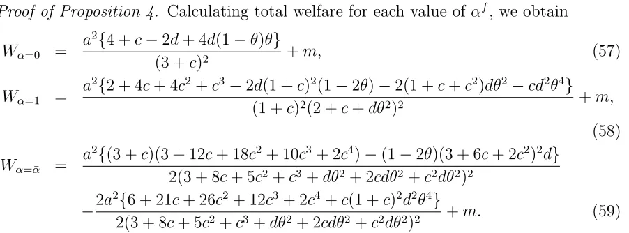
Proof of Proposition 4. Calculating total welfare for each value of αf_{, we obtain}

Wα=0 =

a2_{{4 +c−2d+ 4d(1−θ)θ}}

(3 +c)2 +m, (57)

Wα=1 =

a2_{{2 + 4c+ 4c}2_+c3_{−2d(1 +c)}2_{(1−2θ)−2(1 +c+c}2_)dθ2_−cd2_θ4_} (1 +c)2_{(2 +c+dθ}2₎2 +m,

(58)

Wα= ¯α =

a2_{{(3 +c)(3 + 12c+ 18c}2_{+ 10c}3_{+ 2c}4_{)−(1−2θ)(3 + 6c+ 2c}2₎2_d} 2(3 + 8c+ 5c2_+c3_+dθ2_{+ 2cdθ}2_+c2_dθ2₎2

−2a

2_{{6 + 21c+ 26c}2_{+ 12c}3_{+ 2c}4_{+c(1 +c)}2_d2_θ4_}

2(3 + 8c+ 5c2_+c3_+dθ2_{+ 2cdθ}2_+c2_dθ2₎2 +m. (59)

According to Figure 2.6, total welfare as well as local welfare B is unchanged in region

II. In region III, it is necessary to compareW_|α=1 with W|α=0. The result is given by

W_|α=1−W|α=0 =−

2a2_(1−dθ2_{)Y3(c, d, θ)}

(1 +c)2_{(3 +c)}2_{(2 +c+dθ}2₎2, (60)

where

Y3(c, d, θ) = ₋1 + 2c+c2+d(1 +c)2(5 + 2c)(1₋θ)2+d(3 + 3c+ 3c2+c3)θ2

Therefore, whether W_|α=1 or not is larger than W|α=0 depends on the sign of 1−dθ2.

In regions I and IV, it is necessary to compare W_|α=1 with W|α= ¯α. The result is

shown by

W_|α=1−W|α= ¯α =−

a2_{{c−(1 + 2c)dθ}2_{}Y4(c, d, θ)}

2(1 +c)2_{(2 +c+dθ}2₎2_{(3 + 8c+ 5c}2_+c3_+dθ2 _{+ 2cdθ}2_+c2_dθ2₎2, (62)

where

Y4(c, d, θ) =17c+ 47c2+ 41c3+ 15c4+ 2c5 + 3(1 +c)2d2θ4

+ (1 +c)2d(1₋θ)2_{12 + 31c+ 20c2 + 4c3 + (5 + 10c+ 4c2)dθ2_}

+ (7 + 24c+ 25c2+ 12c3+ 2c4)dθ2 >0. (63)

Therefore, whether or not wB|α=1 is larger than wB|α= ¯α depends on the sign of c−(1 +

2c)dθ2_.

References

B´arcena-Ruiz, J. C. and Garz´on M. B., (2006), “Mixed oligopoly and environmental policy”,Spanish Economic Review, 8: 139-160.

Beladi, H. and Chao, C.-C., (2006), “Does privatization improve the environment?”,

Economics Letters, 93: 343-347.

B¨os, D., (1991),Privatization: a theoretical treatment, Clarendon Press, Oxford.

Cato, S., (2008), “Privatization and the environment”,Economics Bulletin, 12: 1-10.

Fern´andez, J. A. and Fern´andez-Stembridge, L., (2007),China’s state-owned enterprise

reforms – an industrial and CEO approarch, Routledge.

Fjell, K. and Heywood, S., (2004), “Mixed oligopoly, subsidization and the order of firm’s moves: the relevance of privatization”,Economics Letters, 83: 411-416.

Fjell, K. and Pal, D., (1996), “A mixed oligopoly in the presence of foreign private firms”, Canadian Journal of Economics, 29: 737-743.

Ichikawa, Y. and Fujita, S., (1995), “An analysis of wet deposition of sulfate using a trajectory model for East Asia”,Water, Air, and Soil Pollution, 85: 1927-1932.

Kato, K., (2006), “Can allowing to trade permits enhance welfare in mixed oligopoly?”,

Journal of Economics, 88: 263-283.

Kato, K., (2010), “Emission Quota versus Emission Tax in a Mixed Duopoly”, forth-coming in Environmental Economics and Policy Studies.

Lu, Y., (2006), “Endogenous timing in a mixed oligopoly with foreign competitors: The linear demand case”, Journal of Economics, 88: 49-68.

Matsumura, T. (1998), “Partial privatization in mixed duopoly”, Journal of Public Economics,70: 473-483.

Matsumura, T., (2003), “Stackelberg mixed duopoly with a foreign competitor”, Bul-letin of Economic Research, 55: 275-287.

Nagase, Y. and Silva, E. C. D., (2007), “Acid rain in China and Japan: a game-theoretic analysis”, Regional Science and Urban Economics, 37: 100-120.

Naito, T. and Ogawa, H., (2009), “Direct versus indirect environmental regulation in a partially privatized mixed duopoly”,Environmental Economics and Policy Studies,

Ohara, T., Uno, I., Wakamatsu, S., and Murano, K., (2001), “Numerical simulation of the springtime transboundary air pollution in East Asia”,Water, Air, and Soil Pollution, 130: 295-300.

Ohori, S., (2006a), “Optimal environmental tax and level of privatization in an inter-national duopoly”, Journal of Regulatory Economics, 29: 225-233.

Ohori, S., (2006b), “Trade liberalization, consumption externalities and the environ-ment: a mixed duopoly approach”,Economics Bulletin, 17: 1-9.

Wang, L. F.S. and Wang, J., (2009), “Environmental taxes in a differentiated mixed duopoly”, Economic Systems, 33: 389 – 396.

Region A Region B wind

RegionA Region B

θQ 0

Q wind

1 Case (h)

Case (f)

(1₋θ)Q θQ

Q

0

1

(1₋θ)Q

Figure 1: Two cases of ownership are considered in this paper. Case (h): firm 1 is owned

by private investors from region A; Case (f): firm 1 is owned by private investors from

θ

d 0

1

I

1 2

θ=√1 2d

wh

B|α=αh > wh

B|α=1

wh

B|α=1 > whB|α=αh

II

Figure 2: Comparisons between wh

θ

d 0

1

I

1 2

θ = ¯θ

θ =√₂1_d

Wh

|α=αh > Wh|_α=1

Wh_|

α=1 > Wh|α=αh

II

III

Figure 3: Comparison between Wh_|

θ

d 0

1

c

1+2c

3+2c

2(1+c) 1

θ =√ c d(1+2c) θ=√1_d θ =√_2d3+2₍₁₊c_c)

αf _{= ¯α (Partial privatization)}

αf _{= 0 (Full privatization)}

αf _{= 1 (No privatization)}

I

II

III

IV

θ

d 0

1

I

c

1+2c

3+2c

2(1+c) 1

θ =√ c d(1+2c) θ =√1

d

θ =√ 3+2c

2d(1+c)

wf_B|α= ¯α> wfB|α=1

wf_B|α=1 > wfB|α=0

Unchanged

II

III

IV

w_Bf_|α=1 > wBf|α= ¯α

Figure 5: Comparisons betweenw_Bf_|α=1,w f

B|α=αh, andwf

θ

d 0

1

I

c

1+2c

3+2c

2(1+c) 1

θ =√_d(1+2c _c) θ =√1

d

θ =√ 3+2c

2d(1+c)

Wf

|α= ¯α > Wf|α=1

Wf_|

α=1 > Wf|α=0

Unchanged

II

III

IV

Wf_|

α=1 > Wf|α= ¯α

Figure 6: Comparisons betweenWf