© 2016, IRJET | Impact Factor value: 4.45 | ISO 9001:2008 Certified Journal
| Page 1848
A comprehensive study on different approximation methods of
Fractional order system
Asif Iqbal and Rakesh Roshon Shekh
P.G Scholar, Dept. of Electrical Engineering, NITTTR, Kolkata, West Bengal, India
P.G Scholar, Dept. of Electrical Engineering, NITTTR, Kolkata, West Bengal, India
---***---Abstract -
Many natural phenomena can be moreaccurately modeled using non-integer or fractional order calculus. As the fractional order differentiator is mathematically equivalent to infinite dimensional filter, it’s proper integer order approximation is very much important. In this paper four different approximation methods are given and these four approximation methods are applied on two different examples and the results are compared both in time domain and in frequency domain. Continued Fraction Expansion method is applied on a fractional order plant model and the approximated model is converted to its equivalent delta domain model. Then step response of both delta domain and continuous domain model is shown.
Key Words: Fractional Order Calculus, Delta operator Oustaloup approximation method, Modified Oustaloup approximation method, Continued Fraction Expansion (CFE) method, Matsuda approximation method, Illustrative examples.
1. INTRODUCTION
Fractional calculus is the generalization of traditional calculus and it deals with the derivatives and integrals of arbitrary order (i.e. non-integer).It is a 300 years old topic and the idea started when L’Hospital asked Leibniz about ½ order derivative in 1695.Leibniz in a letter dated September 30, 1695 (The exact birthday of fractional calculus) replied that It will lead to an apparent paradox, from which one day useful consequences will be drawn [11]. In 1695 Leibniz mentioned derivatives of “general order” in his correspondence with Bernoulli. After that many scientist worked on it but the actual progress started in June 1974 when B.Ross organized the first conference on application of fractional calculus at the University of New Haven.
Most of the natural phenomena are generally fractional but their fractionality is very small so that it can be neglected. But for accurate modelling fractional calculus is more suited than traditional calculus. Due to the lack of solution methods of fractional differential equations scientists and mathematicians had used the integer order model before late nineties’ but now there are some methods for approximation of fraction derivative and integrals. So it can be easily used in areas of science (e.g. control system, circuit theory etc.). It has been found that fractional controller is more effective than integer order controller and it gives better performance and flexibility. Fractional order system is
infinite dimensional (i.e. infinite memory). So for analysis, controller design, signal processing etc. these infinite order systems are approximated by finite order integer order system in a proper range of frequencies of practical interest [1], [2].
1.1 FRACTIONAL CALCULAS: INRODUCTION
Fractional Calculus [3], is a generalization of integer order calculus to non-integer order fundamental operatorl
D
t,where 1 and t is the lower and upper limit of integration and the order of operation is
.
0
)
(
)
(
0
)
(
1
0
)
(
)
(
R
dx
R
R
dx
d
D
tl t
l (1)
Where
R
is the real part of
. In this paper we consider only those cases where
is a real number, i.e.
R
. There are some commonly used definitions are Grunwald-Letnikov definition, Riemann-Liouville definition and Caputo definition.The Riemann-Liouville definition of the fractional Integral is given below:
d
x
f
dx
d
m
x
f
D
t
l
m m
t
l
1 ( ))
(
)
(
)
(
1
)
(
(2)For
m
1
m
Where,
p
is the Euler’s gamma function.The Grunwald-Letnikov definition, based on successive differentiation, is given below:
)
(
)
1
(
)
(
)
(
1
lim
)
(
) (
0
0
k
f
x
kh
k
h
x
f
D
h x
k h
t
l
(3)So it can be seen from the above definition that by using the fractional order operator l
D
tf
(x
)
© 2016, IRJET | Impact Factor value: 4.45 | ISO 9001:2008 Certified Journal
| Page 1849
t l m m t l Cx
d
f
m
x
f
D
( 1 )) (
)
(
)
(
1
)
(
(4)For
m
1
m
Let us consider the following fractional order differential equation which represents the dynamics of a system:
)
(
)
(
)
(
)
(
)
(
)
(
0 1 0 1 0 1 0 1t
u
D
b
t
u
D
b
t
u
D
b
t
y
D
a
t
y
D
a
t
y
D
a
m m n n m m n n
(5) Wherea
k,
b
k are real coefficients and
k,
k are positive real numbers. Taking Laplace transform of the above equation and assuming zero initial condition, the fractional order model takes the following form:0 1 0 1 0 1 0 1
)
(
)
(
)
(
s
a
s
a
s
a
s
b
s
b
s
b
s
U
s
Y
s
G
n n m m n n m m
(6)
Where,
L
y
(
t
)
Y
(
s
),
L
u
(
t
)
U
(
s
)
1.2
DELTA OPERATOR
The shift operator model of a system has the form:
k
u
D
k
x
C
k
y
k
u
B
k
x
A
k
x
q
q q q q
(7)At very high frequency
T
0
this model fails becauseI
A
q
&B
q
O
, to overcome this problem Middleton & Goodwin proposed a new operator called Delta operator. It is represented as:
T
kT
f
T
k
f
kT
f
1
(8)
T
q
1
(9)And the corresponding complex variable
is defined as
T
e
T
Z
sT1
1
(10)The delta operator model of a MIMO system is given below
k
u
D
k
x
C
k
y
k
u
B
k
x
A
k
x
(11)And it relates with the continuous model and shift operator model and continuous time model as:
e
d
T
T A
01
(12)T
I
A
A
A
c q
(13)
T
B
B
B
c
q (14)
C
C
c
C
q (15)D
D
c
D
q (16) WhereA
c,
B
c,
C
c&
D
c are the state space matrix of continuous time model. At very high sampling frequency delta domain model converges to its continuous counterpart. Thus the system theory is unified by using delta operator based approach.1.3 OUSTALOUP APPROXIMATION METHOD
Oustaloup approximation [5] is widely used in fractional order control. This approximation method is based on the recursive distribution of poles and zero’s. It approximates the basic fractional order operator
s
(
0
1
)
to a integer order rational form within a chosen frequency band. Let
l,
h
the desired frequency band is. Even within that frequency band both gain and phase have ripples, which decreases as the order of approximation increases. The method is given below:
N N k k ks
s
K
s
' (17)
Where,
N
Order of approximation
K
Gain
h 1 2 1 2 1 '
Zeros
N N k l h l k
1 2 1 2 1
N N k l h l kPoles
1.4
MODIFIED OUSTALOUP APPROXIMATION
In Oustaloup approximation method the quality of approximation is poor near the edges of desired frequency band. To overcome this problem the authors modify this approximation method [6], and present a new modified method, known as modified oustaloup approximation method. This method gives very good fitting in the whole frequency range of interest. This approximation is only valid for
0
1
. For higher order derivative, 2.3s
e.g. , the approximation method should be applied to 0.3© 2016, IRJET | Impact Factor value: 4.45 | ISO 9001:2008 Certified Journal
| Page 1850
original derivative is approximated by 2 0.3s
s
, for fractionalintegrals,
s
s
s
0.6
0.4 . The algorithm is given below:
N N k k k h hs
s
d
s
b
s
d
s
b
ds
K
s
' 2 21
(14)Where,
N N k k k n l
b
d
K
'
2 1 2 '
N k n l kb
d
2 1 2
N k n h kd
b
After extensive calculation it has been found that for the best fitting the values of b and d is 10 and 9.
1.5
CFE APPROXIMATION
The CFE approximation [7-9], is given below:
)
(
)
(
)
(
)
(
)
(
)
(
,
1 1 0 1 1 0
mm m m m m mm m m m m mq
s
q
s
q
p
s
p
s
p
s
G
s
(15)
Where
m
is the order of approximation andm
i
n
q
n
p
mi(
),
mi(
),
0
,
1
,
,
are the coefficients. These coefficients can be calculated from the following formula.
m i
ii i m m mi
m
n
i
n
i
m
B
n
q
n
p
1
,
1
)
(
)
(
, (16)Where,
B
(
m
,
i
)
= Binomial Coefficients
i)!
(m
i!
m!
u
k = Pochammer symbol
u
(
u
1
)(
u
2
)
(
u
k
1
)
u
0
1
1.6
MATSUDA APPROXIMATION
Matsuda approximation method [10], approximates fractional differential operator into rational model in two steps. First a rational model of the irrational function is obtained by CFE and then it fits the original function in a set of some points which are logarithmically spaced. Assume that the points taken are
p
k,
k
0
,
1
,
2
,
then the approximation method has the following form:
3 2 2 1 1 0 0)
(
a
p
s
a
p
s
a
p
s
a
s
G
(17)Where,
a
i
i(
p
i)
0(
s
)
G
(
s
)
i i i i
a
s
p
s
s
)
(
)
(
1
In this approximation method the sum of total number of zero’s and total no of poles is N (order of approximation).This method has a drawback, if N is odd the approximated transfer function will be improper i.e., there will be one more zero’s than poles.
2. ILLUSTRATIVE EXAMPLE
In this section two examples are shown and the results of different approximation methods are presented and compared. In the first example, fractional derivative 0.4
s
isapproximated and the results are compared. In the second example different approximation methods are applied on a fractional order transfer function and the results are studied both in time domain and in frequency domain Then CFE method is applied on second example to obtain an approximated transfer function and the results are shown and model reduction is done on the approximated transfer function and its equivalent model is obtained in delta domain. Then its delta domain response is shown.
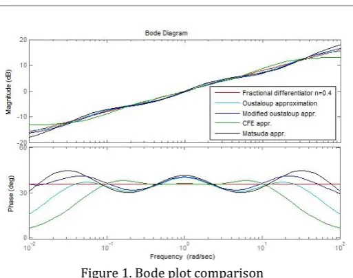
Example 1: Here pure fractional order differentiator is approximated by different approximation methods within the frequency of 0.01 to 100 rad/sec. The order of approximation is 3.The results of different approximation methods are below:
Oustaloup approximation:
31
.
6
14
.
77
74
.
41
1
74
.
41
14
.
77
31
.
6
1
3 22 3
s
s
s
s
s
s
g
(18)Modified Oustaloup approximation:
207
.
4
1220
14320
7809
9
.
226
6
.
177
7413
137660
1243
08
.
10
2
5 4 3 22 3 4 5
s
s
s
s
s
s
s
s
s
s
g
(19) CFE approximation:42
.
11
65
.
63
43
.
42
5
.
2
5
.
2
43
.
42
65
.
63
42
.
11
3
3 22 3
s
s
s
s
s
s
g
(20)Matsuda approximation:
01
.
10
6
.
163
01
.
83
1
01
.
83
6
.
163
01
.
10
4
3 22 3
s
s
s
s
s
s
g
(21)© 2016, IRJET | Impact Factor value: 4.45 | ISO 9001:2008 Certified Journal
| Page 1851
Figure 1. Bode plot comparisonExample 2: In this example approximated model of a fractional order transfer function is obtained by different approximation methods and the results are compared. The fractional order transfer function given below:
1
288
185
10
1
)
(
3.2 2.5 0.7
s
s
s
s
s
G
(21)Approximation methods are applied on fractional powered terms 0.2 0.5
,
s
s
& 0.7s
and the overall transfer function is calculated. Here the order of approximation is 3 and the frequency range is 0.01 to 100. [image:4.595.36.293.79.281.2]The exact bode diagram of fractional order transfer function and the approximated models are obtained. The responses are presented in figure 2.
Figure 2. Bode plot comparison
The step response of the original model and the different approximation models are obtained. The responses are given in figure 3.
Figure 3. Step response comparison
Using CFE approximation method and taking the approximation order as three the equivalent integer order transfer function within the frequency band 0.01 rad/sec to 100 rad/sec is obtained as below:
0530
.
3
434000
.
1
6400000
.
1
76820000
172500000
217100000
185700000
114100000
43350000
8266000
659000
18020
1
.
142
1883
32120
208000
650800
1058000
935700
448700
108900
11320
5
.
481
781
.
6
)
(
2 3
4 5
6
7 8
9
10 11
12
2 3
4 5
6
7 8
9 10
s
s
s
s
s
s
s
s
s
s
s
s
s
s
s
s
s
s
s
s
s
s
s
G
a(22)
The approximated model has the order of 10. On increasing the order of approximation more accurate approximation will be obtained but the order of the model will be very large. So model reduction is very important.
Using the algorithm presented in [10], the reduced model is obtained as:
0497
.
0
636
.
1
4406
.
0
003066
.
0
00926
.
0
0007923
.
0
2 3
2
s
s
s
s
s
s
G
r (23) [image:4.595.41.285.505.690.2]© 2016, IRJET | Impact Factor value: 4.45 | ISO 9001:2008 Certified Journal
| Page 1852
Figure 4. Step response comparisonThe equivalent delta domain model for the sampling period 0.01 is obtained using the Delta Transform. The resulting models for sampling period 0.01 is given below:
0496
.
0
6327
.
1
456
.
0
0031
.
0
0093
.
0
0008
.
0
2 3
2
1
G
(24)The step response of the two delta domain models are obtained. The responses are shown in figure 5.
Figure 5. Step response in Delta domain
3. CONCLUSIONS
In this paper a comprehensive study on four different approximation methods of fractional order operator is presented with two different illustrative examples. The simulation results are also given so that one can easily study the quality of approximation of different approximation methods. If the order of approximation is increased the approximated model will converge to original model and
more accurate fitting will be obtained. The equivalent delta domain model and simulation results are also given. From the results it is hard to tell which one of the approximation methods is the best. Even though some of them are better than others for some characteristics. The relative merits of different approximation methods depend on whether one is more interested in accurate frequency behavior or in accurate time responses.
REFERENCES
[1] M. Khanra, J. Pal, and K. Biswas, "Rational approximation and analog realization of Fractional order transfer function with multiple Fractional powered terms," Asian Journel of Control, Vol. 15 , No. 3, pp. 1-13, May 2013.
[2] M. Khanra, J. Pal, and K. Biswas, "Reduced order approximation of MIMO Fractional order system," IEEE journel on emerging and selected topics in Circuits and Systems, Vol. 3, No. 3, September 2013.
[3] M.D. Ortigueira," Fractional Calculas for Scientists and Engineers,"Volume 84, London, New York : Springer, 2011.
[4] R. Matusu," Application of Fractional order calculas to control theory," International Journel of mathematical models and methods in applied science, Issue 7, volume 5, 2011.
[5] A. Oustaloup, F. Levron, B. Mathieu, and F.M. Nanot," Frequency-band complex noninteger differentiator: characterization and synthesis," IEEE Trans. Circuits Syst. 1, vol. 47, pp. 25-39,2000.
[6] D. Xue, C. Zhao, and Y.Q. Chen," A Modified approximation method of Fractional order system," in proc. of the IEEE International conference on Mechatronics and Automation, Luoyang, China, June 25-28, 2006.
[7] G. Maione," High-Speed digital realization of Fractional operators in Delta domain," IEEE Trans. on Automatic control, Vol. 56, No. 3, March 2011.
[8] G. Maione," Continued fractions approximation of the impulse response of fractional-order dynamic systems," IET Control Theory Appl., Vol. 2, No. 7, pp. 564-572, 2008.
[9] G.Maione,"Concerning Continued fractions representation of noninteger order digirtal differentiator," IEEE signal proc. Letters, Vol. 13, No. 12, December 2006.
[10] D.Y. Xue and Y.Q. Chen," Sub-optimal
H
2 rational approximations to fractional order linear systems," In proc. of the ASME 2005 International Design Engineering Technical Conferences & Computers and Information in Engineering Conference, Long Beach, California, USA, 2005.[11] Y. Q. Chen, I. Petras and D. Xue, “Fractional Order Control
[image:5.595.40.287.438.615.2]© 2016, IRJET | Impact Factor value: 4.45 | ISO 9001:2008 Certified Journal
| Page 1853
BIOGRAPHIES
Asif Iqbal received the B. Tech degree in electronics and communication engineering from Techno India College of Technology, Kolkata, India, in 2013. Since august 2014, he is pursuing M. Tech in Mechatronics engineering in National Institute of Technical Teachers’ Training and Research, Kolkata, and working in the area of fractional order systems approximations and delta domain realization of fractional order systems.
Rakesh Roshon Shekh received the B. Tech degree in electronics and communication engineering from Asansol Engineering college, Asansol, India, in 2013. Since august 2014, he is pursuing M. Tech in Mechatronics engineering in National Institute of Technical Teachers’ Training and Research, Kolkata, and working in the area of fractional order systems approximations and delta domain realization of fractional order systems.