THE PERFORMANCE OF DIRECTIONAL FLOODING ROUTING PROTOCOL FOR UNDERWATER SENSOR NETWORKS
NUR ASFARINA BINTI IDRUS
A thesis submitted in partial
fulfillment of the requirement for the award of the Degree of Master of Electrical Engineering
Faculty of Electrical and Electronic Engineering Universiti Tun Hussein Onn Malaysia
ABSTRACT
ABSTRAK
CONTENTS
TITLE i
DECLARATION ii
DEDICATION iii
ACKNOWLEDGEMENT iv
ABSTRACT v
ABSTRAK vi
CONTENTS vii
LIST OF TABLES xi
LIST OF FIGURES xii
LIST OF SYMBOLS AND ABBREVIATIONS xiv
LIST OF APPENDICES xvi
LIST OF PUBLICATIONS xvii
CHAPTER 1 INTRODUCTION 1
1.1 Background and History 1
1.2 Motivation/Problem Statements of the Study 2
1.3 Aim of the Study 3
1.4 Objectives of the Study 3
2.2 Underwater Wireless Sensor Network Theory 5 2.2.1 Different between Terrestrial and Underwater
Wireless Sensor Networks 7
2.2.2 Propagation Model 8
2.2.3 Network Architecture 10
2.3 Description of Previous Research 11
2.3.1 Routing Schemes 11
2.3.1.1 VBR (Vector based forwarding) 12 2.3.1.2 FBR (Focused beam routing) 14 2.3.1.3 DBR (Depth based routing) 15 2.3.1.4 H2-DAB (Hop-by-hop dynamic addressing
based routing) 15 2.3.1.5 DFR (Directional Flooding based routing) 16 2.3.1.6 EUROP (Energy efficient routing protocol) 17
2.4 Performance Evaluation 18
2.4.1 Packet Delivery Ratio 19
2.4.2 End-to-end Delay 19
2.4.3 Energy Consumption 19
2.5 Summary of Chapter 20
CHAPTER 3 METHODOLOGY 21
3.1 Introduction 21
3.2 Design Procedure 21
3.2.1 Underwater Acoustic Channel 23 3.2.2 A Protocol Stack for Underwater Acoustic
Communications 26
3.3 Software Implementation 30
3.3.1 OMNeT++ Overview 30
3.3.1.1Hierarchical Modules 33
3.3.1.2Module Types 33
3.3.1.4Modeling of Packet Transmissions 34
3.3.1.5Parameters 36
3.3.1.6Topology Description Method 36
3.3.2 The NED Language 36
3.3.3 Simple Modules 38
3.3.4 Compound Modules 39
3.3.5 Internal Architecture 40
3.3.6 Model Repositories 42
3.3.6.1MIXIM Framework 42 3.3.6.2INET Framework 42
3.4 Summary of Chapter 43
CHAPTER 4 SIMULATION 44
4.1 Introduction 44
4.2 OMNeT++, INET and MIXIM Framework
Installation Guide 44
4.3 Getting Started in OMNeT++ IDE 47
4.4 Import and Build MIXIM-INET 53
4.5 Simulation Scenarios 55
4.5.1 Network Architecture 56 4.5.2 Directional Flooding Routing Operation 57
4.6 Summary of Chapter 58
CHAPTER 5 RESULTS AND DATA ANALYSIS 59
5.1 Introduction 59
5.2 Evaluation Results 59
5.3 Triangular Topology Results 60
5.3.1 Static Sink and Number of Nodes Scenario 60
5.4 Random Topology Results 62
5.4.1 Node Speeds Scenario 62
5.4.2 Number of Sinks Scenario 64
5.4.3 Depth Scenario 66
5.5 Discussion 67
6.4 Significant of Findings 70
6.5 Future Works 71
REFERENCES 72
APPENDIX 75
LIST OF TABLES
2.1 Communication requirements of UWSNs 6
2.2 Comparison between terrestrial and UWSNs 7 2.2 (continued)Comparison between terrestrial and UWSNs 8 2.3 Theoretical comparison of acoustic, EM and optical
waves in seawater environments 9
2.4 Performance comparison of UWSN protocols 18
LIST OF FIGURES
2.1 Cluster-based underwater acoustic sensor network model 6
2.2 The OSI reference model 11
2.3 Classification of the routing protocols for UWSNs 12 2.4 VBF routing protocol which uses single pipeline for
each node 13
2.5 A virtual pipelines for each forwarder by HH-VBF 13 2.6 (a) Procedure of finding next hop node in the FBR,
(b) The region of forwarder node selection in the FBR 14 2.7 Assigning HopIDs with the help of Hello packets in
H2-DAB 15
2.8 Packet forwarding in DFR protocol 16
3.1 Flowchart of overall project 22
3.2 Model structure in OMNeT++ 30
3.3 The OMNeT++ simulation process flowchart 32
3.4 Message transmission 35
3.5 Message sending over multiple channels 35
3.6 Example simple module in .cc file 38
3.7 Example simple module in NED file 39
3.8 Example of compound module 40
3.9 Logical architecture of an OMNeT++ simulation 41 3.10 Screenshot of TKENV as user interfaces in OMNeT++ 42
4.1 Mingwenv file 45
4.2 Installation INET 46
4.3 Installation MIXIM 46
4.4 Final installation 47
4.5 OMNeT++ IDE simulator 48
4.7 New OMNeT++ project 49
4.8 The initial contents 49
4.9 Ini file options 50
4.10 Selecting the specified network 50
4.11 Run configurations setup 51
4.12 Executable simulation environment 52
4.13 Simulation GUI 52
4.14 Create a new workspace 53
4.15 Import folder 53
4.16 Browse mixim-inet folder 54
4.17 C/C++ build for both framework 54
4.18 (a) The illustration model of triangular topology in UWSN (b) The illustration model of random
topology in UWSN 56
4.19 The illustration model of DFR protocol 57 5.1 Packet delivery ratio with different transmission range
in DFR 61
5.2 Energy consumption with different transmission range
in DFR 61
5.3 End-to-end delay with different transmission range
in DFR 62
5.4 Packet delivery ratio for node mobility speed in DFR 63 5.5 End-to-end delay for node mobility speed in DFR 64 5.6 Packet delivery ratio with different number of sinks
in DFR protocols 65
5.7 End-to-end delay with different number of sinks in DFR
protocols 65
LIST OF SYMBOLS AND ABBREVIATIONS
f - Frequency
% - Percentage
°C - Degree Celsius
a - Frequency-dependent parameter
An - The coefficients
B(OH)3 - Boric acid
dA - Sender’s depth
dB - Decibels
dB - Receiver’s depth
e() - Signal loss due to random noise or error E() - The function of wave effects in nodes
h(s) - The scale factor function
hw - The wave height in meters
k - The spreading factor
Kbps - Kilo bit per seconds
kHz - Kilo Hertz
km - Kilometers
kW - Kilo Watt
lw - The ocean wavelength in meters
m - Meters
m(f, s, dA, dB) - The propagation loss without random and periodic
MgSO4 - Magnesium sulphate
MHz - Mega Hertz
pH - Potential of hydrogen
PL(t) - The propagation loss from node A to B
RN - The random number from a Gaussian distribution
S - Euclidean distance between nodes A and B
Tw - The wave period in seconds
w(t) - Periodic function to approximate signal due to wave α - The absorption coefficient factor
2D - Two dimension architecture
3D - Three dimension architecture
DBR - Depth Based Routing
DFR - Directional Flooding Based Routing
EM - Electromagnetic wave
EUROP - Energy Efficient Routing Protocol
FBR - Focused Beam Routing
H2-DAB - Hop-by-hop Dynamic Addressing Based Routing HH-VBF - Hop-by-hop vector based forwarding
HTML - Hyper Text Markup Language
IDE - Integrated Development Environment
MAC - Medium Access Control
MMPE - Monterrey Miami Parabolic Equation
NED - Network Description Language
OMNeT++ - Objective Modular Network Testbed in C++
OSI - Open Systems Interconnection
PSU - Practical Salinity Unit
RREP - Route Request
RREQ - Route Reply
RTS - Request to Send
TKENV - The graphical runtime environment UWSNs - Underwater Wireless Sensor Networks
LIST OF APPENDICES
APPENDIX TITLE PAGE
A DFR Protocol Simulation Setup in Omnetpp.ini File 75 B Table B.1: Gantt Chart of Master’s Project 1 78 B Table B.2: Gantt Chart of Master’s Project 2 79
C Proceeding papers 80
LIST OF PUBLICATIONS
Proceedings:
1CHAPTER 1
INTRODUCTION
2
1.1 Background and History
Wireless sensor networks became popular research area at the end of 20th century and covers only terrestrial applications. The deep oceans are harsh environments for human to explore and the existing sensing technologies do not meet the need for easy deployable low cost equipments. The underwater world has always fascinated human beings and almost two third of the Earth is covered by the largely unexplored vastness of the seas and has attracted human’s attention.
The traditional approach to ocean monitoring is to deploy oceanographic sensors, record the data, and recover the instruments which spend lots of time receiving the recorded information. Additionally, if failure occurs before recovery, all the data would be lost. The ideal solution is to establish real-time communication between the underwater instruments and a control center within a network configuration (Sozer, Stojanovic et al. 2000, Xiao 2009). Also, the concept of an ad-hoc and sensor networks for underwater is very attractive, because it can be helpful and easily extend the range of current acoustic modems. It also offers distributed communications with less deployment time.
researched and solved. The development of Underwater Wireless Sensor Networks (UWSNs) has never been more interesting than in the last few years. Here, we attempt to analyze behaviour of UWSN based on the technology developed during the last decade in terrestrial wireless sensor networks (TWSNs). Although it has a very similar functionality, UWSNs exhibit several architectural differences with respect to the terrestrial ones, which are mainly due to the characteristic of transmission medium (seawater) and the signal employed to transmit the data, which is the acoustic ultrasound signals (Akyildiz, Pompili et al. 2007).
The underwater acoustic channel differs from radio channels in many aspects. The available bandwidth of the underwater acoustic channel is limited and also dependent on both range and frequency. In acoustic communications, shorter links have access to a wider bandwidth due to the specific features of acoustic propagation and noise. The sensors are battery powered so power efficiency is a critical issue for underwater sensor networks as well. In addition, extremely long delay in the underwater acoustic channel could lead to collapse of traditional terrestrial routing protocols because of limited response waiting time. According to circumstances, designing a suitable network routing protocol in underwater environment is urgent. Sensor nodes with wireless communication can be deployed under the sea level. The sensors detect and transfer the data from the bottom level to the top level (Chun-Hao and Kuo-Feng 2008).
1.2 Motivation/Problem Statements of the Study
Underwater Wireless Sensor Networks (UWSNs). Study aims are typically identified in relation between performance achievements of the protocol in end-to-end delay, packet delivery ratio and energy consumption can be suitable for the underwater medium.
1.4 Objectives of the Study
The objectives of the study are:
(i) Investigate the architecture and performances of routing protocol for UWSN. (ii) Analyze the suitability of the protocol for the sub aquatic transmission
medium in fresh water or seawater.
(iii) Evaluate the performances of the protocol by considering the following metric; end-to-end delay, packet delivery ratio and energy consumption.
1.5 Scope and Limitations of the Study
1.6 Outlines of the thesis
The outlines of this thesis are organized as follows:
Chapter 1: This chapter covers the background and history of underwater wireless sensor networks, motivation or problem statements, aims, objectives, scope and limitations and outlines of the thesis.
Chapter 2: This chapter deals with review related literature of others research or previous studies which conclude theoretical and results. It also clarified, justified and compared to results based on related research.
Chapter 3: In this chapter comprises the methodology or approaches in order to achieve the aims of the study. It shows procedure or protocols used in completion of this study.
Chapter 4: The simulation implementation and setup are described in this chapter. Metrics and parameters are also discussed and explained during simulation process.
Chapter 5: Results and data analysis are addressed through simulation using OMNeT++. Simulation output and the results of comparative study are shown and explained in this chapter.
3CHAPTER 2
LITERATURE REVIEW
4
2.1 Introduction
This chapter provides a survey of an existing routing protocol that is used for underwater sensor networks. The surveys include the basic underwater sensor network theory, the comparison between terrestrial and UWSN characteristics, propagation model and suitable network architecture. The surveys then focus to the various routing protocols, metrics and their performances. Comparative analysis are done base on various metrics such as the packet delivery ratio, end-to-end delay and energy consumption. The rest of the chapter is organized as follows. Section 2.2 describes underwater wireless sensor networks theory. Section 2.3 outlines the description of previous research. Section 2.4 provides a brief performance metrics of the existing protocols. The chapter is summarized in section 2.5.
2.2 Underwater Wireless Sensor Networks Theory
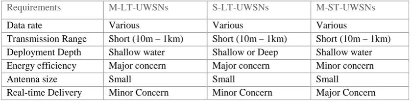
sensor nodes (buoyancy controlled or fixed at sea floor) (Jun-Hong, Jiejun et al. 2006). The later usually mobile since the cost of deploying or recovering fixed sensor nodes is typically prohibitive for short term time critical applications (Lanbo, Shengli et al. 2008). Obviously, different types of UWSNs have different communication requirements as summarized in Table 2.1.
Table 2.1: Communication requirements of UWSNs (Lanbo, Shengli et al. 2008)
Requirements M-LT-UWSNs S-LT-UWSNs M-ST-UWSNs
Data rate Various Various Various
Transmission Range Short (10m – 1km) Short (10m – 1km) Short (10m – 1km) Deployment Depth Shallow water Shallow or Deep Shallow water Energy efficiency Major concern Major concern Minor concern
Antenna size Small Small Small
Real-time Delivery Minor Concern Minor Concern Major Concern
Underwater sensor networks consist of a group of sensor nodes anchored to the sea bed that are acoustically connected together and to other underwater gateways through clustering or cell. Clusters contain sensors and sinks where sensors are connected to sinks within each cluster. These connections may be multiple hops or direct paths. The signals shared at each sink within a cluster are transmitted to the surface stations through a vertical link. The surface station will handle multiple parallel communications with the sinks deployed underwater by acoustic transceivers (Thumpi.R 2013).
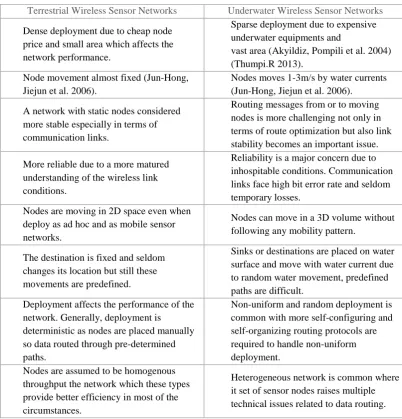
[image:20.595.159.480.553.721.2]applications. But in last several years, an underwater sensor network has found an increasing use in a wide range of networks. Table 2.2 is shown the comparison between both applications.
Table 2.2: Comparison between terrestrial and UWSNs (Ayaz, Baig et al. 2011) (Kheirabadi and Mohamad 2013)
Terrestrial Wireless Sensor Networks Underwater Wireless Sensor Networks
Dense deployment due to cheap node price and small area which affects the network performance.
Sparse deployment due to expensive underwater equipments and
vast area (Akyildiz, Pompili et al. 2004) (Thumpi.R 2013).
Node movement almost fixed (Jun-Hong, Jiejun et al. 2006).
Nodes moves 1-3m/s by water currents (Jun-Hong, Jiejun et al. 2006).
A network with static nodes considered more stable especially in terms of communication links.
Routing messages from or to moving nodes is more challenging not only in terms of route optimization but also link stability becomes an important issue.
More reliable due to a more matured understanding of the wireless link conditions.
Reliability is a major concern due to inhospitable conditions. Communication links face high bit error rate and seldom temporary losses.
Nodes are moving in 2D space even when deploy as ad hoc and as mobile sensor networks.
Nodes can move in a 3D volume without following any mobility pattern.
The destination is fixed and seldom changes its location but still these movements are predefined.
Sinks or destinations are placed on water surface and move with water current due to random water movement, predefined paths are difficult.
Deployment affects the performance of the network. Generally, deployment is deterministic as nodes are placed manually so data routed through pre-determined paths.
Non-uniform and random deployment is common with more self-configuring and self-organizing routing protocols are required to handle non-uniform deployment.
Nodes are assumed to be homogenous throughput the network which these types provide better efficiency in most of the circumstances.
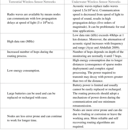
Table 2.2 (continued): Comparison between terrestrial and UWSNs (Ayaz, Baig et al. 2011) (Kheirabadi and Mohamad 2013)
Terrestrial Wireless Sensor Networks Underwater Wireless Sensor Networks
Radio waves are available by means nodes can communicate with low propagation delays at speed of light (3 𝑥𝑥 108m/s).
Acoustic waves replace radio waves (speed 1.5𝑥𝑥103m/s). Communication speed is decreased from speed of light to speed of sound, results in high
propagation delays (five orders of magnitude). It can be problematic for real time applications.
High data rate (MHz)
Low data rate (kHz) exceeds 40kbps at 1 km distance. Moreover, the attenuation of acoustic signal increases with frequency and range (Ayaz and Abdullah 2009). Increased number of hops during the
routing process.
Number of hops depends on depth of the monitoring are normally 4 until 7 hops.
Low energy consumption.
High energy consumption due to longer distances (consequence of sparse nodes deployment) and complex signal processing. The power required to transmit may decay with powers greater than two of the distance.
Large batteries can be used and can be replaced or recharged with ease.
Battery power is limited and usually cannot be easily replaced or recharged. The routing protocols should adopt a mechanism of power down during the communication and use minimum retransmission.
Nodes are less error prone and can continue to work for longer time.
Nodes are more error prone and can die due to fouling or corrosion or leave the working area. More reliable and self recovering routing algorithms are required.
2.2.2 Propagation Model
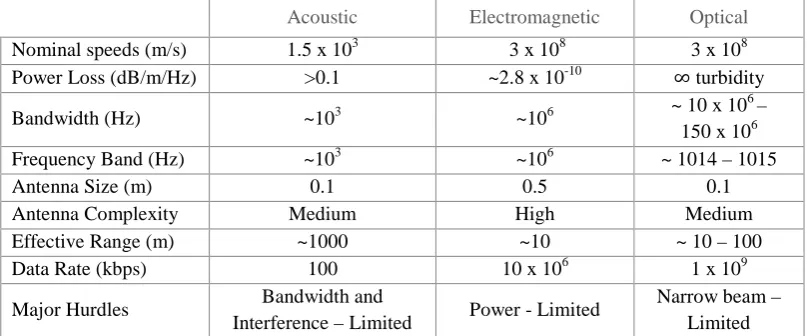
[image:22.595.120.530.131.548.2]research in the years 1950 to 1970. Seawater is a conductive medium with large electromagnetic signal attenuations, which increase with frequency (Balanis 2012). There have been several attempts to develop underwater Electromagnetic wave (EM) signal propagation based communication models as shown in Table 2.3. Underwater communications simulation requires modeling the acoustic wave’s propagation while a node tries to transmit data to another one. An acoustic communications are classified by different features but it can hardly exceed 40kbps at a range of 1km. The speed of sound generally depends on water properties which is temperature, pressure and salinity. The speed of sound near the ocean surface is 4 times faster than the speed of sound in air with the increase of practical salinity unit (PSU), temperature and depth. Hence, the ocean salinity in seawater is defined as ionic salt concentration with 35.5 PSU in average salinity.
Table 2.3: Theoretical comparison of acoustic, EM and optical waves in seawater environments (Uribe and Grote 2009)
Acoustic Electromagnetic Optical
Nominal speeds (m/s) 1.5 x 10³ 3 x 10⁸ 3 x 10⁸
Power Loss (dB/m/Hz) >0.1 ~2.8 x 10⁻¹⁰ ∞ turbidity
Bandwidth (Hz) ~103 ~106 ~ 10 x 10
6 –
150 x 106
Frequency Band (Hz) ~103 ~106 ~ 1014 – 1015
Antenna Size (m) 0.1 0.5 0.1
Antenna Complexity Medium High Medium
Effective Range (m) ~1000 ~10 ~ 10 – 100
Data Rate (kbps) 100 10 x 106 1 x 10⁹
Major Hurdles Bandwidth and
Interference – Limited Power - Limited
2.2.3 Network Architecture
The network architecture of UWSN can be described in the form of two dimensional and three dimensional structures. Static two dimensional UWSNs for ocean bottom monitoring consist of sensor nodes that are anchored to the bottom of the ocean. Typical applications may be environmental monitoring or underwater tectonic plates monitoring. Static three dimensional UWSNs for ocean column monitoring including networks of sensors whose depth can be controlled and may be used for surveillance applications or ocean phenomena monitoring (Akyildiz, Pompili et al. 2004) (Zhang, Xiao et al. 2009). Underwater sensors may be organized in cluster based architecture and be interconnected to one or more underwater gateways (uw-gateways) by means of wireless acoustic links. Underwater gateways introduce devices in charge of relaying data from the ocean bottom network to a surface station. They are equipped with a long range vertical transceiver used to relay data to a surface station and with a horizontal transceiver used to communicate with the sensor nodes for sending commands signals and collecting and aggregating the data. The surface station is equipped with an acoustic transceiver that is able to handle multiple parallel communications with the deployed uw-gateways, and with a long-range radio transmitter and/or satellite transmitter that needed to communicate with an onshore sink and/or to a surface sink (Akyildiz, Pompili et al. 2004) (Pompili, Melodia et al. 2009).
2.3 Description of Previous Research
For the last few years many researchers have shown interest in the fields of underwater sensor network. There are several previous researches that contribute to this area specifically in the subtopic of routing, end-to-end delay, energy efficiency and packet delivery ratio. Each contributed paper used different routing protocols, show the performance results and software that was used to solve the problem in underwater sensor networks.
2.3.1 Routing Schemes
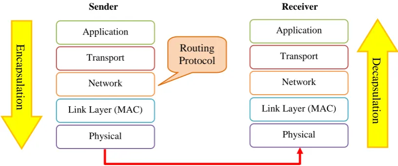
[image:25.595.115.524.527.698.2]Routing protocol is a fundamental issue for any network and considered to be in charge for discovering and maintaining the routes (Wahid 2010). Underwater environment is related to physical layer while the routing techniques issue is related to network layer of the OSI (Open Systems Interconnection) reference model as shown in Fig.2.2. Most researchers have proposed various types of routing protocol to get the performance metrics in network layer according to the requirement with different applications in underwater environment.
Figure 2.2: The OSI reference model
Application
Transport
Network
Link Layer (MAC)
Physical
Application
Transport
Network
Link Layer (MAC)
Physical Routing Protocol E nc aps ul at ion D ecap su lat io n
Sender Receiver
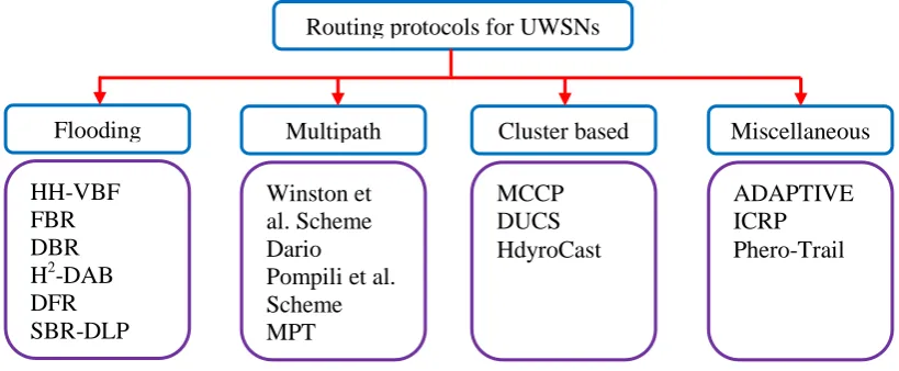
Routing layer of underwater sensor networks employ in various approaches by means flooding based, multipath based, cluster based and miscellaneous (Wahid 2010). Fig. 2.3 shows the classification of the selected protocols. The selection of the protocols follows the criterion of the most citation and recently proposed approaches. In flooding approach, the transmitters send a packet to all nodes within the transmission range. This protocol is simple and provides network knowledge while the main disadvantage is that nodes many transmit duplicate packet and resulted in more energy been consumed. In multipath based approach, it established more than one path from a source node towards a sink node. This formation augments the robustness and reliability. Clustering based approach means, the sensor nodes are grouped together in a cluster. The group consists of clusterhead and non-clusterhead. Clusterhead collects data from members of the clusterhead and generate transmission schedule. On the other hand, non-clusterhead nodes aggregate the sensed data and transmit data packets to the clusterhead. This thesis focused only on flooding based protocols for UWSNs.
Figure 2.3: Classification of the routing protocols for UWSNs (Wahid 2010)
2.3.1.1 VBR (Vector based forwarding)
In VBF (Xie, Zhou et al. 2010), data packets are forwarded along redundant and interleaved paths from the source to sink where it mitigate the problems of packet losses and node failures. Forwarding path from sender to target is nominated by the routing vector. All nodes which received the packet compute their positions by
Routing protocols for UWSNs
Flooding Multipath Cluster based Miscellaneous
HH-VBF FBR DBR H2-DAB DFR SBR-DLP
Winston et al. Scheme Dario
source and the destination nodes and packet delivery is occurred along this pipe.
Figure 2.4: VBF routing protocol which uses single pipeline for each node (Kheirabadi and Mohamad 2013)
Figure 2.5: A virtual pipelines for each forwarder by HH-VBF (Kheirabadi and Mohamad 2013)
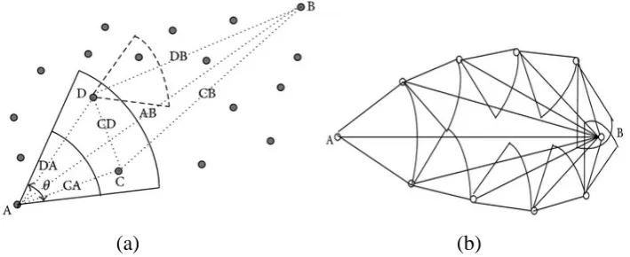
[image:27.595.221.424.356.468.2]2.3.1.2 FBR (Focused beam routing)
FBR (Jornet, Stojanovic et al. 2008) protocols for acoustic sensor networks are intended to avoid unnecessary flooding of broadcast queries. Overall expected throughput is significantly reduced by overburdened networks due to uncertain location information of nodes. Other than that, the location of intermediate nodes is not required. Routes are established dynamically during the traverse data packet for its destination and the decision about the nest hop is made at each step on the path after the appropriate nodes have proposed themselves.
[image:28.595.156.511.304.449.2](a) (b)
Figure 2.6: (a) Procedure of finding next hop node in the FBR, (b) The region of forwarder node selection in the FBR (Kheirabadi and Mohamad 2013)
which is use depth sensors. It senses own relative current position from the surface and place its value in the header and then broadcasts when a node wants to send a data packet. The receiving node calculates its own depth position and compares this value with the value embedded in the packet. The packet is forwarded if it is smaller and otherwise the packet will be discarded. The process is repeated until the packet reaches the destination. The main disadvantage of this protocol is that in sparse and high density areas, the performance is affected by packet loss and inefficient memory usage.
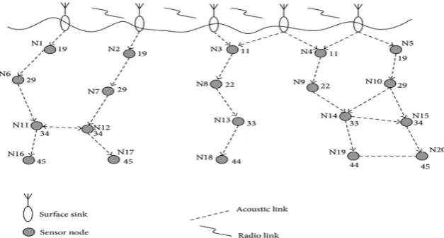
2.3.1.4 H2-DAB (Hop-by-hop dynamic addressing based routing)
[image:29.595.183.497.552.720.2]These protocols are assumes that are multiple buoys on the water surface which collect data of nodes anchored at the bottom of the sea and deployed at different depths. Sensor data is sent towards the water surface in a greedy fashion. The flooding based approach is employed along with the utilization of unique IDs to each sensor nodes. A hop ID illustrates the distance of hop count from a sink node towards the sensor node. In H2-DAB protocol, multi sink architecture is taken into account where consider the transmitted packets delivered to the destination if any of the sinks receives the packet correctly.
Furthermore, H2-DAB (Ayaz and Abdullah 2009) has many advantages by means it does not require any specialized hardware, require no dimensional location information and handle node movements easily without maintaining complex routing tables. The multi-hop routing problems still exists as it is based on multi-hop architecture, where nodes near the sinks drain more energy because they are used more frequently.
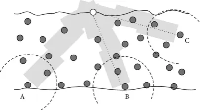
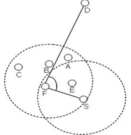
2.3.1.5 DFR (Directional Flooding based routing)
[image:30.595.272.405.515.652.2]The DFR (Daeyoup and Dongkyun 2008) (Shin, Hwang et al. 2012) protocol enhances reliability by packet flooding technique. The packets are transmitted in a restricted flooding zone where the zone area is selected based on an angle formed by the vectors. The vector between the receiver and the sender of the packet and another formed is the vector between the receiver and the destination node. The assumption is that all nodes know about its own location, location of one next hop and destination. Link quality is the foundation for deciding the forwarding nodes. This protocol rectifies the void problem by the selection of at least one node to transmit the data packet towards the sink but it can still exist if the sending node cannot find a next hop closer to the sink as reverse transmission of data packet is impossible.
amount of energy consumption by reducing broadcast hello messages. The depth sensor will eliminate the requirement of hello messages for control position, which can be helpful for increasing the energy efficiency. These sensor nodes are deployed at different depths in order to observe the events occurring at different locations in the network. Further, every node is anchored at the bottom of the ocean and equipped with a floating module that can inflated by a pump. This electronic module that resides on the node helps push the node towards the surface and return back to its initial position.
Table 2.4: Performance comparison of UWSN protocols (Wahid 2010, Ayaz, Baig et al. 2011)
Protocol
Scheme Mobility
Packet delivery ratio End-to end delay Energy consumption Network dimension Number
of nodes Depth
VBF (Xie, Zhou et al. 2010)
Sink fixed and node mobile (0-3m/s)
Medium Low Low
1000m x 1000m x 500m (3D area) From 500 to 4000 500m HH-VBF (Xie and Connectic ut 2008) Sink and
node fixed High Low Low
1000m x 1000m x 500m (3D area) 500 to 3000 nodes 500m FBR (Jornet, Stojanovic et al. 2008) Sink fixed and node mobile (0-3m/s)
Medium Low Medium
200km2 (square area) 100 active nodes n/a DBR (Yan, Shi et al. 2008) Sink (RF) and node mobile (1m/s, 5m/s and 10 m/s)
High Low Medium
500m x 500m x 500m (3D area)
200
nodes 500m
H2-DAB (Ayaz and Abdullah 2009)
Sink and
node fixed High Low Low
1500m x 1500m x 1500m (3D area) 300 (anchor & floating) 1500 m DFR (Shin, Hwang et al. 2012) Sink and
node fixed High Low Low
3000m x 4000m (2D area)
41 nodes n/a
EUROP (Chun-Hao and Kuo-Feng 2008) Sink and
node fixed Medium Low Low
150m x 150m x 150m (3D area)
1000
nodes 150m
2.4 Performance Evaluation
to the destination (sender) compared to the number of packets that have been sent out by the sender. These redundant packets are considered as only one distinct packet whether a packet may reach the sinks multiple times. Illustrates the level of delivered data to the destination:
∑ 𝑁𝑁𝑁𝑁𝑁𝑁𝑁𝑁𝑁𝑁𝑁𝑁 𝑜𝑜𝑜𝑜 𝑝𝑝𝑝𝑝𝑝𝑝𝑝𝑝𝑁𝑁𝑝𝑝 𝑁𝑁𝑁𝑁𝑝𝑝𝑁𝑁𝑟𝑟𝑟𝑟𝑁𝑁𝑁𝑁 ∑ 𝑁𝑁𝑁𝑁𝑁𝑁𝑁𝑁𝑁𝑁𝑁𝑁 𝑜𝑜𝑜𝑜 𝑝𝑝𝑝𝑝𝑝𝑝𝑝𝑝𝑁𝑁𝑝𝑝 𝑠𝑠𝑁𝑁𝑠𝑠𝑠𝑠
The greater value of packet delivery ratio means the better performance of the protocols.
2.4.2 End-to-end Delay
This time delays are an average time taken by a data packet to arrive in the destination. It also includes the delay caused by route discovery process and the queue in the data packet transmitter. Only the data packets that successfully delivered to destinations that counted.
∑(𝑅𝑅𝑁𝑁𝑝𝑝𝑁𝑁𝑟𝑟𝑟𝑟𝑁𝑁 𝑝𝑝𝑟𝑟𝑁𝑁𝑁𝑁 − 𝑆𝑆𝑁𝑁𝑠𝑠𝑠𝑠 𝑝𝑝𝑟𝑟𝑁𝑁𝑁𝑁) ∑𝑁𝑁𝑁𝑁𝑁𝑁𝑁𝑁𝑁𝑁𝑁𝑁 𝑜𝑜𝑜𝑜 𝑝𝑝𝑜𝑜𝑠𝑠𝑠𝑠𝑁𝑁𝑝𝑝𝑝𝑝𝑟𝑟𝑜𝑜𝑠𝑠𝑠𝑠
The lower value of it means the better performance of the protocol.
𝑃𝑃𝑝𝑝𝑝𝑝𝑝𝑝𝑁𝑁𝑝𝑝 𝐿𝐿𝑜𝑜𝑠𝑠𝑝𝑝=𝑝𝑝ℎ𝑁𝑁 𝑝𝑝𝑜𝑜𝑝𝑝𝑝𝑝𝑡𝑡 𝑠𝑠𝑁𝑁𝑁𝑁𝑁𝑁𝑁𝑁𝑁𝑁 𝑜𝑜𝑜𝑜 𝑝𝑝𝑝𝑝𝑝𝑝𝑝𝑝𝑁𝑁𝑝𝑝𝑠𝑠 𝑠𝑠𝑁𝑁𝑜𝑜𝑝𝑝𝑝𝑝𝑁𝑁𝑠𝑠 𝑠𝑠𝑁𝑁𝑁𝑁𝑟𝑟𝑠𝑠𝑑𝑑 𝑝𝑝ℎ𝑁𝑁 𝑠𝑠𝑟𝑟𝑁𝑁𝑁𝑁𝑡𝑡𝑝𝑝𝑝𝑝𝑟𝑟𝑜𝑜𝑠𝑠 𝑃𝑃𝑝𝑝𝑝𝑝𝑝𝑝𝑁𝑁𝑝𝑝 𝐿𝐿𝑜𝑜𝑠𝑠𝑝𝑝= 𝑁𝑁𝑁𝑁𝑁𝑁𝑁𝑁𝑁𝑁𝑁𝑁 𝑜𝑜𝑜𝑜 𝑝𝑝𝑝𝑝𝑝𝑝𝑝𝑝𝑁𝑁𝑝𝑝 𝑠𝑠𝑁𝑁𝑠𝑠𝑠𝑠 − 𝑁𝑁𝑁𝑁𝑁𝑁𝑁𝑁𝑁𝑁𝑁𝑁 𝑜𝑜𝑜𝑜 𝑝𝑝𝑝𝑝𝑝𝑝𝑝𝑝𝑁𝑁𝑝𝑝 𝑁𝑁𝑁𝑁𝑝𝑝𝑁𝑁𝑟𝑟𝑟𝑟𝑁𝑁𝑁𝑁
However, the lower value of the packet lost means the better performance of the protocol.
2.4.3 Energy Consumption
affected by network dynamics, large propagation delays and high error probability of acoustic channels. The direct way to resolve this problem is to generate energy by the sensors themselves. The probably method we can used is current movement or chemistry method to generate power to recharge battery. Efficient routing protocol and communication method can contribute to these issues. Energy consumption is the one of the biggest constraints of the wireless. Sensor nodes often use limited energy sources such as batteries. Therefore, the implementation of energy saving techniques is needed.
2.5 Summary of Chapter
CHAPTER 3
METHODOLOGY
5
3.1 Introduction
This chapter is described about the methodology that will be used in this research. The overview for all stages is discussed in flowchart form to summarize the progress of this project.
3.2 Design Procedure
The procedure of designing this study represented the flowchart shown in Fig. 3.1. In the earlier stages, the problems, objectives and scopes of the study identified where are related with title of project by approval from supervisor. After that, there will be lot information by reviewing the previous projects and references such as journal, thesis, survey or review papers that very useful for this research done. While understanding the fundamental and theory background by means underwater wireless sensor networks, routing protocol and performance metrics also will be involved.
end-to-end delay and energy consumption. This part is designed and simulates using OMNeT++ software and analyzes the simulation results. Finally, conclude the enhanced results to achieve the objectives of this project.
Figure 3.1: Flowchart of overall project
Yes Start
End Identified the problem
Discuss with supervisor Select title of projects
Change title
Seek information and knowledge about underwater
wireless sensor networks
Review the previous projects
Explore OMNeT++ software
Study routing protocols in underwater environment
Change routing protocols
Discuss and analyze the results
Conclude Simulation process (performance evaluation) No
Yes No
Master Project 1
to electromagnetic propagation through the atmosphere modeling sound behaviour in dissipative transmission medium, such as seawater. Propagation delay, interferences and signal attenuations are characterized in this study. Basically, an underwater environment is formed with the cooperation of several network sensor nodes that establish and maintain the network through bidirectional acoustic links. Every node is able to send or receive messages from/to intermediate nodes in the network, and also forward messages to remote sink in case of multi-hop networks.
The main aspects of acoustic signals in UWSNs are given by: (1) the acoustic wave velocity is close to 1500m/s and so the communication links will suffer from large and variable propagation delays and relatively large motion-induced Doppler effects; (2) phase and magnitude fluctuations lead to higher bit error rates by using the forward error correction codes (FEC); (3) the attenuation observed in the acoustic channel increases when the frequency increases, thus produced a serious bandwidth constraint; (4) multipath interference in underwater acoustic communications is severe due mainly to the surface waves or vessel activity, being a serious problem to attain good bandwidth efficiency (Hwee-Xian and Seah 2007, Llor and Malumbres 2012). Simulating underwater medium requires modeling the acoustic signal while a node tries to transmit data to another node. In these subsections, several underwater acoustic channels represent in UWSNs.
A. Urick Description and Thorps Formula
The theory of the sound propagation is properly described by Urick (Urick 1983), as a regular molecular movement in an elastic substance that propagates to adjacent particles. A sound wave can be considered as the mechanical energy that is transmitted by the source from particle to particle, being propagated through the ocean at the speed of sound. The attenuation is often the most limiting factor in acoustic propagation where the amount depends on propagation medium and frequency. In seawater, attenuation comes from the viscosity of pure water, the relaxation of magnesium sulphate (MgS04) molecules above 10 - 500kHz and boric
Thorp (Llor and Malumbres 2012) is defined as the sound intensity decrease through the path between the source and destination nodes. The absorption coefficient factor α depends on the sound frequency f. The proposed acoustic attenuation expression is represented as follows (Lucani, Médard et al. 2008):
A (d, f)=dk α(f)d (3.1)
where k is the spreading factor (1 for cylindrical, 1.5 for practical spreading and 2 for spherical), a is a frequency-dependent parameter (Lurton 2002)
10 log𝛼𝛼(𝑜𝑜) =0.11𝑜𝑜2 1+𝑜𝑜2 +
44𝑜𝑜2
4100+𝑜𝑜2+ 2.75𝑥𝑥10−4𝑥𝑥𝑜𝑜2+ 0.003 (3.2)
where 𝛼𝛼(𝑜𝑜) is given in dB/km and f is in kHz. The absorption coefficient is the major factor that limits the maximum usable bandwidth at a given distance as it increases very rapidly with frequency. This formula is under a temperature of 4 °C, a salinity of 35 %, a pH of 8.0 and a depth of about 50m. It suitable for low frequency 30 kHz region and it approximate 7.609dB/km measurement results for proposed frequency.
B. Monterrey Miami Parabolic Equation (MMPE)
The Monterey-Miami Parabolic Equation model (Llor and Malumbres 2012) is used to predict underwater acoustic propagation using a parabolic equation which is closer to the Helmholtz equation (wave equation); this equation is based on Fourier analysis. The sound pressure is calculated in small incremental changes in range and depth, forming a grid. It incorporates randomness and wave motion to the approximation, using a dynamic propagation loss calculation. The authors show that small changes in depth and node distances can drive to big differences in the path loss as a result of the ocean wave’s motion impact on acoustic propagation. The propagation loss formula based on the MMPE model is the following one:
REFERENCES
Akyildiz, I. F., D. Pompili and T. Melodia (2004). "Challenges for efficient communication in underwater acoustic sensor networks." SIGBED Rev. 1(2): 3-8.
Akyildiz, I. F., D. Pompili and T. Melodia (2007). "State of the art in protocol research for underwater acoustic sensor networks." SIGMOBILE Mob. Comput. Commun. Rev. 11(4): 11-22.
Ayaz, M. and A. Abdullah (2009). Hop-by-Hop Dynamic Addressing Based (H2-DAB) Routing Protocol for Underwater Wireless Sensor Networks. Information and Multimedia Technology, 2009. ICIMT '09. International Conference on.
Ayaz, M. and A. Abdullah (2009). Underwater wireless sensor networks: routing issues and future challenges. Proceedings of the 7th International Conference on Advances in Mobile Computing and Multimedia. Kuala Lumpur, Malaysia, ACM: 370-375.
Ayaz, M., I. Baig, A. Abdullah and I. Faye (2011). "Review: A survey on routing techniques in underwater wireless sensor networks." J. Netw. Comput. Appl. 34(6): 1908-1927.
Balanis, C. A. (2012). Advanced Engineering Electromagnetics, Wiley.
Chun-Hao, Y. and S. Kuo-Feng (2008). An energy-efficient routing protocol in underwater sensor networks. Sensing Technology, 2008. ICST 2008. 3rd International Conference on.
Daeyoup, H. and K. Dongkyun (2008). DFR: Directional flooding-based routing protocol for underwater sensor networks. OCEANS 2008.
Hwee-Xian, T. and W. K. G. Seah (2007). Distributed CDMA-based MAC Protocol for Underwater Sensor Networks. Local Computer Networks, 2007. LCN 2007. 32nd IEEE Conference on.
Jornet, J. M., M. Stojanovic and M. Zorzi (2008). Focused beam routing protocol for underwater acoustic networks. Proceedings of the third ACM international workshop on Underwater Networks. San Francisco, California, USA, ACM: 75-82.
Jun-Hong, C., K. Jiejun, M. Gerla and Z. Shengli (2006). "The challenges of building mobile underwater wireless networks for aquatic applications." Network, IEEE 20(3): 12-18.
Kheirabadi, M. T. and M. M. Mohamad (2013). "Greedy Routing in Underwater Acoustic Sensor Networks: A Survey." International Journal of Distributed Sensor Networks 2013: 21.
Lanbo, L., Z. Shengli and C. Jun-Hong (2008). "Prospects and problems of wireless communication for underwater sensor networks." Wirel. Commun. Mob. Comput. 8(8): 977-994.
Llor, J. and M. P. Malumbres (2012). "Underwater Wireless Sensor Networks: how do acoustic propagation models impact the performance of higher-level protocols?" Sensors 12(2): 1312-1335.
Lucani, D. E., M. Médard and M. Stojanovic (2008). "Underwater acoustic networks: channel models and network coding based lower bound to transmission power for multicast." Selected Areas in Communications, IEEE Journal on 26(9): 1708-1719.
Lurton, X. (2002). An Introduction to Underwater Acoustics: Principles and Applications, Springer.
Min, H., Y. Cho and J. Heo (2012). Enhancing the reliability of head nodes in underwater sensor networks.
Pompili, D., T. Melodia and I. F. Akyildiz (2006). Deployment analysis in underwater acoustic wireless sensor networks. Proceedings of the 1st ACM international workshop on Underwater networks. Los Angeles, CA, USA, ACM: 48-55.
Pompili, D., T. Melodia and I. F. Akyildiz (2009). "Three-dimensional and two-dimensional deployment analysis for underwater acoustic sensor networks." Ad Hoc Netw. 7(4): 778-790.
Rodoplu, V. and A. A. Gohari (2010). "maC protocol design for underwater networks." Underwater Acoustic Sensor Networks: 179.
Shin, D., D. Hwang and D. Kim (2012). "DFR: an efficient directional flooding-based routing protocol in underwater sensor networks." Wirel. Commun. Mob. Comput. 12(17): 1517-1527.
Soo Young, S. and P. Soo Hyun (2008). Omnet++ Based Simulation for Underwater Environment. Embedded and Ubiquitous Computing, 2008. EUC '08. IEEE/IFIP International Conference on.
Sozer, E. M., M. Stojanovic and J. G. Proakis (2000). "Underwater acoustic networks." Oceanic Engineering, IEEE Journal of 25(1): 72-83.
Thumpi.R, M. R. B., Sunilkumar S.Manvi (2013). "A Survey on Routing Protocols for Underwater Acoustic Sensor Networks." International Journal of Recent Technology and Engineering (IJRTE) 2(2).
Uribe, C. and W. Grote (2009). Radio Communication Model for Underwater WSN. New Technologies, Mobility and Security (NTMS), 2009 3rd International Conference on.
Urick, R. J. (1983). "Principles of underwater sound. 1983." McGraw-HiII, New York, London.
Varga, A. and R. Hornig (2008). An overview of the OMNeT++ simulation environment. Proceedings of the 1st international conference on Simulation tools and techniques for communications, networks and systems & workshops, ICST (Institute for Computer Sciences, Social-Informatics and Telecommunications Engineering).
Wahid, A. a. D., K. (2010). "Analyzing Routing Protocols for Underwater Wireless Sensor Networks." International Journal of Communication Networks & Information Security 2(No. 4).
Connecticut.
Xie, P., Z. Zhou, N. Nicolaou, A. See, J.-H. Cui and Z. Shi (2010). "Efficient vector-based forwarding for underwater sensor networks." EURASIP J. Wirel. Commun. Netw. 2010: 1-13.
Yan, H., Z. J. Shi and J.-H. Cui (2008). DBR: depth-based routing for underwater sensor networks. Proceedings of the 7th international IFIP-TC6 networking conference on AdHoc and sensor networks, wireless networks, next generation internet. Singapore, Springer-Verlag: 72-86.