Observer based Control for Time–varying Delay Systems with Delay dependence

Observer-based Control for Time–varying Delay Systems

with Delay-dependence

Pin-Lin Liu

Department of Automation Engineering Institute of Mechatronoptic System, Chienkuo Technology University, Changhua, 500, Taiwan *Corresponding Author: [email protected]

Copyright © 2013 Horizon Research Publishing All rights reserved.

Abstract

This paper is concerned with the problem of observer control of a class of time-varying delay systems with delayed measurements. By using information on delay derivative, improved asymptotic stability conditions for time-delay systems are presented. Unlike previous methods, upper bound of delay derivative is taken into consideration, even if this upper bound is larger than or equal to 1. We develop delay-dependent method for designing linear observer controllers, thus ensuring global uniform asymptotic stabilization for any time delay no larger than a given bound. Numerical examples are given to illustrate effectiveness and less conservatism of obtained stability conditions.

Keywords

Observer controller, time-varying delay system, linear matrix inequality (LMI), integral inequality approach (IIA), maximum allowable delay bound (MADB)

1. Introduction

Time-delay systems constitute a special class of dynamical systems that are commonly found in chemical and biochemical engineering systems, as well in other fields of engineering. Time-delay usually lead to unsatisfactory performance and is frequently a source of instability. Stability properties of time-delay systems have been extensively studied in literature, mainly in applied mathematics and control theory related journals [1-8, 10-13, 15-18, 20-24]. It can be claimed that any real-life system has time delay associated with it. The delay in a system may be due to one or more of the following causes: (i) measurement of system variables, (ii) physical properties of the equipment used in the system, and (iii) signal transmission (transport delay) [20]. For systems with time-varying delays, the above mentioned literature usually demand that the upper bound of the derivative of delays must be smaller than 1. If the upper bound of the derivative of delays is larger than 1, the results in [8, 10, 11,22] are not applicable.

It is well known that a static (or dynamic) output

controller, which uses only the output for feedback, is more practical to deal with time-varying delay systems [7, 14]. In particular, the observer-based output feedback controller, which is a dynamic output feedback controller, can on-line estimate the system states.The control of such systems has been thoroughly studied. One of the major difficulties in implementing a control law is that all of the state variables of the system are required for the controller synthesis. However, in the most practical situations, this condition is rarely satisfied and an observer has to be building up in order to estimate the state variables from the output and the input measurements. Observer analysis of such kind of systems has been the subject of numerous papers and monographs [2, 4, 5, 9, 18, 21, 23; 24] and the references therein. Referring to the extensive results on stabilization and observation of time-delay systems, the conditions under which stabilizing feedbacks exist are classified into two possible categories: delay independent conditions and delay-dependent ones [17]. Even, delay-independent conditions do not take into account the size of the delay and may lead to robust control design, the delay-dependent results reveal less conservative than delay independent conditions. Nevertheless, in most cases, a small delay is tolerable to maintain stability by output feedbacks.

The present paper addresses problem of stabilization for linear time-varying delay systems under observer controller. A delay dependent robust stabilization condition is derived based on linear matrix inequalities (LMIs). The stabilization analysis is derived in three steps: (i) applying a state-observer controller to reconstruct an approximation of the unavailable state from the available input and output of the systems, (ii) the choosing of Lyapunov–Krasovskii functional with linear matrix inequality (LMI) techniques and integral inequality approach (IIA) in the designed observer controller and (iii) finally, a maximum allowable delay bound which ensures that the class of time-varying delay system with observer controller considered in this paper is stabilizable for any h is determined by solving an optimization problem.

2. Stability Description and

Preliminaries

Let us consider the system described by the following linear differential- difference equation

0 1

( ) ( ) ( ( )) ( ),

x t =Ax t +Ax t h t− +Bu t _t>0,

(1a) ( ) ( ),

y t =Cx t (1b)

where ( )_{x t ∈R}n _{is the state vector of the system;} 0, , ,1 B C n n

A A _∈R× _{are constant matrices; Time delay, ( ),h t} is a time-varying continuous function that satisfies

0≤h t( )≤h and ( )h t ≤hd, (2)

where hand hdare given positive constants.

In this control system, we assume that ( A0,B) is controllable, i.e. the process state x(t) can be determined on the basis of control input ( )u s for s t≤ . For system (1) subject to delayed measurement, if all the states are not measurable, design an observer controller as follows:

0 1

ˆ ( ) ( ),

ˆ( ) ˆ( ) ˆ( ( )) ( ) [ ( ) ˆ( )],

u t Kx t

x t Ax t Ax t h t Bu t L y t Cx t

= −

= + − + + − (3)

such that the closed-loop system is stable, where K is the controller gain matrix and L is the observer gain matrix.

Introducing the observer error ˆ ( ) ( ) ( ).

e t =x t −x t (4) Combining (1), (2) and (3), we can get

1

( ) e ( ) e ( ( )), e t et et h t

x =Ax +A x − t >0, (5) where

( ) [ ( ) ( )], (e ( )) [ ( ( )) (e ( ))]

T T T T T T

e t t t e t h t t h t t h t

x = x x − = x − −

and

0 1

1

0 1

0

, .

0 0

e e

BK BK

A A

A _LC A

A A

−

   

=_{ } =_{ }

−

   

Before embarking on main results, the following lemmas are introduced, which play important roles in the proof of the main results. First, Lemma 1 induces the integral inequality approach (IIA).

Lemma 1 [16]. For any positive semi-definite matrices:

11 12 13

12 22 23

13 23 33

0,

T T T

X

X

X

X

_X

_X

_X

X

X

X









=

_

_

≥









(6a)

the following integral inequality holds:

33 ( )

( )

11 12 13

12 22 23

13 23

( )

( )

( )

(

( ))

( )

( )

(

( ))

.

0

( )

t T

t h t

t T T T

t h t

T

T T

s

x s ds

x

X

t

t

h t

s

x

x

x

x t

X

X

X

x t

h t

ds

X

X

X

x s

X

X

− −

−

_∫

≤

−

×





∫

_

_



 





 

₋





 





 





 











(6b)

Secondary, we introduce the following Schur complement which is essential in the proofs of our results. Lemma 2[1]. The following matrix inequality:

( )

( )

0,

( )

( )

T

Q x

S x

x

R x

S





<









(7a)

where _{Q x}( )_=QT( ), ( )_{x R x =R}T( ) and ( )_{x S x depend on affine on}

x

,

_{is equivalent to}

( ) 0,R x < (7b) ( ) 0,

Q x < (7c) and

1

( ) ( ) ( ) ( ) 0.T

Q x S x₋ R− x S x _{< (7d)}

Theorem 1: For given scalars h and hd, this system (5) is asymptotically stabilizable by the observer controller (3) if

there exist symmetric positive-definite matrices P>0, Q>0, R>0,and

11 12 13 12 22 23 13 23 33

0 T

T T

X X X

X X X X

X X X

    =_{ }≥     such that

13 13 11 1 13 23 12

1 23 13 12 23 23 22 1

1

(1

)

0,

T T T T

e e e e

T T T T T

e e d e

e e

P P

Q

h

P

h

h R

A

A

X

X

X

A X

X

X

A

P

h

_h

Q

h

h R

A

X

X

X

X

X

X

A

hR

_A

hR

_A

hR

+

+ +

+

+

−

+

+









=

+

−

+

− −

−

−

+

<

Ω 





−







(8a)

and

33

0.R X− ≥ (8b) Proof: A Lyapunov functional can be constructed as

( ) 0 ( ) ( ) ( ) ( )( ) ( ) ( )( ) ( ) t T T

t e e t h t e e

t T

e e

h t

V x x t P tx x t s Q s dsx t s R s dsd

x x

θ θ

−

− +

= _{+ ∫}

+∫ ∫   (9)

Taking time derivative ( )V t for t∈[0, )∞ along trajectory (5) yields

1 1

1

( ) ( )( ) ( ) ( ) ( ( ))

( ( )) ( ) ( ) ( )

( ( ))(1 ( )) ( ( )) ( ) ( )

( ) ( )

( )( ) ( ) ( ) ( ( ))

T T T

e e e

t e e e e

T T T

e

e e e e

T T

e e e e

t T

e e

t h

T T T

e e e

e e e e

T e

V x x t A P PA x t x t PA x t h t

t h t P t t Q t

x A x x x

t h t h t Q t h t t hR t

x x x x

s R s ds

x x

t P P t t P t h t

x A A x x A x

− = + + − + − + − − − − + −∫ ≤ + + − +   _{ }   1 ( ) 1 1 ( ( )) ( ) ( ) ( )

( ( ))(1 ) ( ( )) ( ) ( )

( ) ( )

( ) ( ) ( ) ( ( ))

( ( )) ( )

( ( ))(1 ) ( ( ))

T T

e e e e

T T

e d e e e

t T

e e

t h t

T T T

e e e

e e e e

T T

e

e e

T T

e d e e

t h t P t t Q t

x A x x x

t h t Q t h t t hR t

x h x x x

s R s ds

x x

P P Q t t P t h t

x A A x x A x

t h t P t

x A x

t h t Q t h t

x h x

− − + − − − − + −∫ = + + + − + − − − − − +       33 33 ( ) ( ) ( ) ( ) ( )( ) ( ) ( ) ( ) . e

t T t T

e e e e

t h t t h t

t hR t

x x

s R s ds s s ds

x X x x X x

− −

−∫ − −∫



   

(10)

From Lemma 1 [16], we obtain

33 ( )

11 12 13

12 22 23

( )

13 23

( )

( )

( )

( )

(

( ))

( )

(

( ))

0

( )

t T

e e

t h t

e

t T T T T

e e e e

t h t

T T

e

s

s ds

x

X

x

t

x

X

X

X

t

t h t

s

t h t

ds

x

x

x

X

X

X

x

s

x

X

X

− −

−∫



 





 



≤

∫



_

−



_{ }

×

_{ }

−

_



 





 











11 12 13 12 22 23 13 23

( )

( )

( )

(

( ))

( )

[ ( )

(

( ))]

(

( ))

( )

(

( ))

(

( ))

(

)

[ ( )

(

( ))]

[ ( )

(

( ))]

( )

[ ( )

(

)]

(

T T

e e e e

T T T

e e e e e

T T

e e e e e

T T

e e e

T T

e e e

t h

t

t h

t h t

x

X

x

x

X

x

t h

t

t h t

t h t

t

x

X

x

x

x

hX x

t h t h

t h t

t h

t

t h t

x

X

x

x

X

x

x

t

t h t

t

x

x

X

x

t

t h

t h

x

x

X

x

≤

+

−

+

−

−

+

−

+

−

−

+

−

−

−

+

−

−

+

−

−

−

11 13 13

12 13 23

23 13

12

22 23 23

( ))

( )[

] ( )

( )[

] (

( ))

(

( ))[

] ( )

(

( ))[

] (

( )).

T T e e T T e e

T T T

e e

T T

e e

t

t h

t

x

X

X

X

x

t h

t h t

x

X

X

X

x

t h t

t

x

hX

X

X

x

t h t

h

t h t

x

X

X

X

x

=

+

+

+

−

+

−

+

−

+

−

+

−

−

−

−

(11)

33 ( )

( )

T

( ) ( )

t T

( )(

) ( ) ,

t t h t e e

V



x

≤

ξ

t

Ξ

ξ

t

−

∫

−

x

_

s R

−

X

x

_

s ds

(12) where T( ) T( ) T( ( ))

e e

t x t x t h t

ξ

=_ − _ and

13 13 11 13 23 1 12 1

23 13 1 12 1 23 23 22 1 1

.

(1

)

T T T T T

e e e e e e e

T T T T T T

e e e d e e

P P

Q

h

h R

P

h

h R

A

A

X

X

X

A A

X

X

A

X

A A

P h

h R

h

Q

h

h R

X

X

A

X

A A

X

X

X

A A

+

+ +

+

+

+

−

+

+

+

+





Ξ = 

₋

₊

₊

₊

_{− −}

₋

₋

₊

₊







From Equation (1) and Schur complement [1], we readily see that V x( ) 0t < holds if Ξ <0 and

R X

−

33

>

0.

Time delay systems (1) are asymptotically stable under observer controller (3).

3. Observer Control Design

In this section, we seek a design method of the observer control for a time-varying delay system. Unfortunately, Theorem 1 does not give a feasible LMI condition for obtaining a state feedback control gains matrices K and L. Hence, we look for another stabilization condition. To this end, we make a congruence transformation and obtain a feasible LMI stability condition. Based on it, we give a design method of an observer controller. The following Theorem 2 gives an LMI-based computational procedure to determine dynamic controls. Then we have the following result.

Theorem 2: For given scalars h and hd, the time-varying delay systems (1) is asymptotically stabilizable by the observer controller (3) if there exist symmetric positive-definite matrices 1

2 0 0, 0 W W   >     11 12 12 22 0, T Z Z Z Z   >     11 12 12 22 0, T U U U U   >  

  matrixTijab≥0 ( ,i j=1,2,3, ,a b=1,2), and any matrix ( 1,2)Yii= with appropriate dimensions such

that

11 12 13

12 22 23

13 23 33

0,

T

T T



Ω

Ω

Ω







Ω =

_

_Ω

_Ω

_Ω

_

<



_Ω

_Ω

_Ω







(13a)

and

3311 3312 1

3312 2 3322

-

-0,

-T

W T

T

W

T

T





≥





−





(13b)

where

1 1 1311 2311 1211 1312 2312 1212

12

1312 2312 1212 1322 2322 1222

0 1 1

1 13 0 2 2 1 1 23 11 1 2

,

,

0

0

,

,

0

T T

T T T

T T T T T T T T T aa aa T T ab bb

h

h

W

A

T

T

T

T

T

T

h

h

T

T

T

T

T

T

h

W A

h

Y B

h

Y B

h

_W

_A

h

_Y

_C

hW A

hW A

−

+

+

−

+

+





=

Ω



₋

₊

₊

₋

₊

₊







−





=

Ω



₋













Ω

Ω



=

=

Ω





Ω



_Ω

_Ω











2311 2311 2211 12 2312 2312 2212

11 22

2312 2312 2212 22 2322 2322 2222

12 11 12 33 12 22

(1

)

(1

)

,

(1

)

(1

)

,

T T d d

T T T T

d d

T

h

h

U

T

T

T

h U

T

T

T

h

h

h

U

T

T

T

h U

T

T

T

h

h

Z

h

Z

h

Z

h

Z

−

−

−

−

+

− −

−

−

+





=

Ω



₋

₋

₋

₋

₊

_{− −}

₋

₋

₊







−

−





=

Ω



₋

₋







0 0 1 1 1311 1311 1111

1 1 11

1 12 1312 1312 1112

0 2 2 0 2 2 22 1322 1322 1122

(1

)

,

(1

)

,

(1

)

.

T T T T

aa d

T

ab d

T

T T T

bb d

B

h

W

A

A

W

Y Y B

h U

T

T

T

B

_Y

_{h U}

_T

_T

h

_T

C

h

W W

C

h U

A

A

Y Y

T

T

T

=

+

−

−

+ −

+

+

+

Ω

=

+ −

+

+

+

Ω

=

+

−

−

+ −

+

+

+

Ω

In this case, observer control gains in (3) is given by 1 1 1

K₌YW− _and 1 2 2.

Proof: In view of Theorem 1, to prove the asymptotic stability of the closed-loop system with control

0 1

ˆ( ) ˆ( ) ˆ( ( )) ( ) [ ( ) ˆ( )]

x t =Ax t +Ax t h t− +Bu t +L y t Cx t− u t( )= −Kx tˆ( ), it suffices to show that there exist symmetric, positive-definite matrices P>0, Q>0 and R>0 such that (8) remains valid. Pre- and post- multiplying both sides of (8) by _{diag P P R{ ,}−1 −1_, −1_{} and letting} 1 1 1 1 11 12

2 12 22

0

, ,

0 T

W U U

W Q U

P P P

W U U

− _{= =}  − − _{= =} 

   

   

11 12 1

12 22 , T Z Z Z

R

Z Z

−  

= =  

 

1 1 _{( , 1,2,3, , 1,2),} ij ijabi j a b

P X P− − ₌T _{= = and}

3311 3312

1

1 1 1

33

33 3312 2 3322

-

-0

-T

R

_W

W T

T

R

P

P

T

W

X

T

T

− −





−

₌

₋

₌





_≥



_{ }

_

_

_



_{ −}

₋









leads to (11). Thus, if W U Z Y Y, , , ,1 2 and Tijab are a set of feasible solution to LMI (13), then K =Y1W1−1,L=Y2W2−1 satisfying (13). This ends the proof.

Remark 1: As in the stabilization problem, the upper bound h which ensure that time delays systems (1) is stabilizable under observer controller law (3) for maximum allowable delay bound (MADB) h can be determined by solving the following quasi-convex optimization problem when the other bound of time delay

h

is known.

Maximize h (14) Subject to linear matrix inequality (13) and W >0, U>0, Z >0, and Tijab≥0.

To show usefulness of our result, let us consider the following numerical examples.

4. Illustrative Examples

Example 1: Consider the following time delay dynamic system as follows:

0 1

( )

( )

(

( ))

( ),

x t



=

A

x t

+

A

x t h t

−

+

Bu t

_{t >0, (15a)}

( )

( ),

y t

=

Cx t

_(15b)

where 0 1

0

1

3

2

1 0

,

,

.

1

1.5

0

1

B C

0 1

A

=



_



_

A

=



_

−

−



_

=

=



_



_

−

−













We assumed that the states of the system are not available. How do we find the maximum allowable delay bound (MADB) h with an observer-based controller to guarantee the system (15) to be asymptotically stable.

Solution: When hd=0,by using the LMI Toolbox in MATLAB (with accuracy 0.01),we solve the inequality (13) employing the quasi-convex optimization (14) to yield

1 2

11 12

22

0.0085 0.0056

0.0110 -0.0132

,

,

0.0056 0.0289

-0.0132 0.0218

0.0417 0.0103

0.0044 -0.0096

,

,

0.0103 0.0615

0.0048 0.0039

0.0157 -0.0056

-0.0056

W

W

U

U

U









=

_

_

=

_

_

















=

_

_

=

_

_









=

11

12 22

1 2

1.4296 -0.0380

,

,

0.0335

-0.0380 1.1605

-0.0056 -0.0055

1.0548 -0.0028

,

,

0.0070 0.0011

-0.0028 1.1037

0.0777 0.0325

,

-0.0245 0.0133

Z

Z

Z

Y

Y









=

























=

_

_

=

_

_













=

_

_

=





0.0234 0.0229

.

0.0129 0.0364













The maximum allowable delay bound (MADB) h is h≤2.1713 and the corresponding controller gain matrix Kand the observer gain matrix L are

9.5939 -0.7300

12.3996 8.5711

,

.

-3.6357 1.1632

11.6443 8.7320

K

=



_



_

L

=



_



_









[image:6.595.119.476.85.377.2]

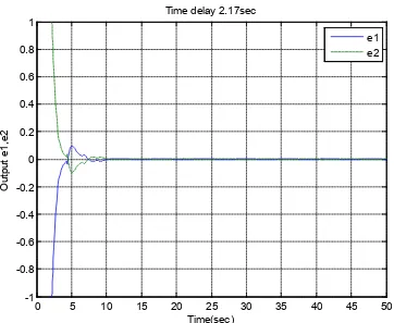
Figure 1. The simulation of the example 1 forh= 2.17 sec

Figure 2. The simulation of the example 1 forh=2.17 sec

0 5 10 15 20 25 30 35 40 45 50

-1 -0.8 -0.6 -0.4 -0.2 0 0.2 0.4 0.6 0.8 1

Time(sec)

O

ut

put

x

1,

x2

Time delay 2.17sec

x1 x2

0 5 10 15 20 25 30 35 40 45 50

-1 -0.8 -0.6 -0.4 -0.2 0 0.2 0.4 0.6 0.8 1

Time(sec)

O

ut

put

e1,

e2

Time delay 2.17sec

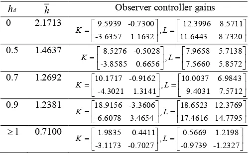
[image:6.595.117.479.414.711.2]

[image:7.595.180.431.156.312.2]

The results of the maximum allowable delay bound (MADB) h for different values of hd are also listed in Table 1. It may be noted that (i) the number of iterations (ii) the control gain associated with the proposed method. It is also clear to show that the maximum allowable delay bound (MADB) h is dependent on different values of .hd The values of hd increases as the maximum allowable delay bound (MADB) h decreases.

Table 1. MADB h for differenthd in Example 1 (Iterations 25)

d

h _h Observer controller gains

0 2.1713 9.5939 -0.7300 _, 12.3996 8.5711 -3.6357 1.1632 11.6443 8.7320

K=_ _ L=_ _

   

0.5 1.4637 8.5276 -0.5028 7.9658 5.7138 ,

-3.8585 0.6656 7.5660 5.8572

K=_{ } L=_ _

   

0.7 1.2692 10.1717 -0.9162 10.0037 6.9843 ,

-4.3021 1.3141 9.4031 7.5712

K=_ _ L=_ _

   

0.9 1.2381 18.9156 -3.3606 18.6523 12.3769 ,

-6.6078 3.4654 17.4616 14.7795

K=_ _ L=_ _

   

1

≥ 0.7100 1.9835 0.4411 _, 0.5669 1.2198 -3.1173 -0.7027 -0.9739 -1.2327

K=_ _ L=_ _

   

Example 2: Consider a linear time delay system with dynamics described by

0 0 0 0 0 0.1

( ) ( ) ( ( )) ( )

1 2 0.2 0.1 1 0

x t =_ _x t +_ _x t h t− +_ _u t

− −

      (16a)

0 1

( )

( ),

1 0

y t

_{= }





_

x t





(16b)

Now, our problem is to calculate the maximum allowable delay bound (MADB) h for which an observer control law, controller gain matrix Kand the observer gain matrix ,L exists to stabilize (16).

Solution: To begin with, forhd=0, equation (16) reduces to the system discussed in [13]. Solving the quasi-convex optimization problem (14), according to the Theorem 2, using the soft-ware package LMI Toolbox, we obtain the corresponding controller gain matrix Kand the observer gain matrix L are -0.8498 -1.2850 ,

5.5876 1.1508

K_{= } _

 

-0.6806 -1.6337 0.5782 0.2456

L=  

 and the maximum allowable delay bound (MADB) is h≤9.8539. The simulation of the above

[image:8.595.121.473.84.380.2]

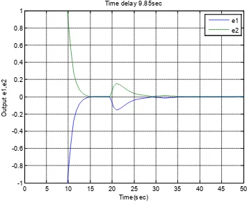
Figure 3. The simulation of the example 2 forh=9.85 sec

Figure 4. The simulation of the example 2 forh=9.85 sec

By taking the parameters hd>1and using the LMI Toolbox in MATLAB (with accuracy 0.01), solving the quasi-convex optimization problem (14), the maximum allowable delay bound (MADB) is h≤3.4440 and the

0 5 10 15 20 25 30 35 40 45 50

-1 -0.8 -0.6 -0.4 -0.2 0 0.2 0.4 0.6 0.8 1

Time(sec)

O

ut

put

x

1,

x2

Time delay 9.85sec

x1 x2

0 5 10 15 20 25 30 35 40 45 50

-1 -0.8 -0.6 -0.4 -0.2 0 0.2 0.4 0.6 0.8 1

Time(sec)

O

ut

put

e1,

e2

Time delay 9.85sec

[image:8.595.121.476.410.705.2]

corresponding controller gain matrix Kand the observer gain matrix L are

-0.8625 -1.6426

_,

-0.6513 -1.7439

_.

0.8318 0.5377

0.2399 0.1378

K

=



_



_

L

=



_



_









Whenhd>1, the stability criteria proposed in [13] cannot be applied to check stabilization of system (16). It is clear that the results obtained in this paper are better than those in [13].

5. Conclusion

The state feedback and observer control problem of a class of time-varying delay systems subject to delayed measurements has been investigated. This problem has been cast into a framework of convex optimization. By constructing a Lyapunov– Krasovskii functional and using a recently developed integral inequality approach, existence conditions for the state feedback and the observer controller have been established. The stability conditions obtained are dependent of the delay values, and are generally less restrictive than those previously presented in the literature. Numerical simulations are given and the results show that the designed observers and controllers are feasible and valid.

REFERENCES

[1] S L. Boyd, E. L. Ghaoui, E. Feron and V. Balakrishnan, Linear Matrix Inequalities in System and Control Theory, PA, Philadelphia: SIAM, 1994.

[2] M. Boutayeb, Observer design for linear time-delay systems, Systems & Control Letters, Vol. 44, No.2, pp. 103-109, 2001.

[3] H. H Choi and M. J. Chung, Observer-based controller design for state delayed linear systems, Automatica, Vol. 32, pp.1073-1075, 1996.

[4] A. Germani, C. Manes, P. Pepe, An asymptotic state observer for a class of nonlinear delay systems, Kybernetika, Vol.37, No.4, pp.459-478, 2001.

[5] A. Germani, C. Manes, P. Pepe, A new approach to state observation of nonlinear systems with delayed output, IEEE Transactions on Automatic Control, Vol. 47, No.1, pp. 96-101, 2002.

[6] Y. He, Q. G. Wang, L. Xie and C. Lin, Further improvement of free-weighting matrices technique for systems with time-varying delay, IEEE Transactions on Automatic Control, Vol.52, No.2, pp.293-299, 2007.

[7] F. H. Hsiao, J. G. Hsieh and M. S. Wu, Determination of the tolerable sector of series nonlinearities in uncertain time-delay systems under dynamical output feedback, Transactions of the ASME Journal of Dynamic Systems, Measurement and Control, Vol. 113, pp.525-531, 1992. [8] C. C. Hu, F. L. Li and X. P. Guan, Observer-based adaptive

control for uncertain time-delay systems. Information Sciences, Vol. 176, pp. 201-214, 2006.

[9] S. Ibrir, Convex optimization approach to observer- based stabilization of uncertain linear systems, Transactions of the

ASME Journal of Dynamic Systems, Measurement and Control, Vol.128, No.4, pp. 989-994, 2006.

[10] S. Ibrir, Observer-based control of a class of time- delay nonlinear systems having triangular structure, Automatica, Vol. 47, pp.388-394, 2011.

[11] Kwon OM, Park JH, Lee SM, Won SC. LMI Optimization approach to observer-based controller design of uncertain time-delay systems via delayed feedback, Journal of Optimization Theory and Applications 2006; 128(1): 103-117, 2006.

[12] J. Leyva-Ramos and A. E. Pearson, Output feedback stabilizing controller for time-delay systems, Automatica, Vol.36, pp.613-621, 2000.

[13] X. Li, CE. de Souza, Output feedback stabilization of linear time-delay systems, in Stability and Control of Time-Delay Systems (L. Dugard, E. I. Verriest) LNCIS, Springer-Verlag, London, Vol.228: 241-258, 1997.

[14] C. Lin, J. L. Wang, G. H. Yang and C. B. Soh, Robust controllability and robust closed-loop stability with static output feedback for a class of uncertain descriptor systems, Linear Algebra and Its Applications, Vol.297, pp.133-55, 1999.

[15] C. Li, Q. G. Wang, T. H. Lee, Y. He and B. Chen Observer-based fuzzy control design for T–S fuzzy systems with state delay, Automatica Vol.44, pp.868-874, 2008.

[16] Liu PL. State feedback stabilization of time-varying delay uncertain systems: A delay decomposition approach, Linear Algebra and Its Applications 2013; 438 (5): 2188-2209.

[17] M. S. Mahmoud, Robust control and filtering for time-delay systems, New-York: Marcel Dekker, 2000.

[18] L.A. Marquez, C. Moog, and M. Velasco Villa, Observability and observers for nonlinear systems with time delay, Kybernetika, Vol. 38, No.4, pp.445 -456, 2002. [19] J. B. Pearson, Compensator design for dynamic optimization,

International Journal of Control, Vol. 9, No.4, pp. 473-482, 1969

[20] T. J. Su and P. L. Liu, Robust stability for linear uncertain time-delay systems with delay-dependence, International Journal of Systems Science, Vol. 24, No.6, pp. 1067-1080, 1993.

[21] Z. Wang, D. P. Goodall and K. J. Burnham, On designing observers for time delay systems with nonlinear disturbances, International Journal of Control, Vol.75, No.11, pp. 803-811, 2002.

[23] S. Xu and P. V. Dooren, Robust filtering for a class of nonlinear systems with state delay and parameter uncertainty, International Journal of Control , Vol.75, No.10, pp.766-774, 2002.