Embedded Adaptive Self-Tuning Control Development
by a Free Toolchain
Gernot Grabmair
∗,
Simon Mayr
Upper Austria University of Applied Sciences, Stelzhamerstrae 23, 4600 Wels, Austria
Copyright c⃝2015 by authors, all rights reserved. Authors agree that this article remains permanently
open access under the terms of the Creative Commons Attribution License 4.0 International License
Abstract
In this study, we present an adaptive self-tuning controller (STC) design for small embedded systems. The new free tool-chain for model based control design is based, among other software, on the open simulator Scilab-XCos. After a very short introduction of model based design terms, this article focuses on the code generator and the other pro-grams of the tool-chain. The design concept is demonstrated by the non-trivial adaptive self-tuning control (STC) of the cart system in simulation and on a real laboratory experiment.Keywords
Open Source, Code Generation, Scilab-XCos, Model Based Control, Adaptive Control, Embedded Systems1
Introduction
Model-Based Design (MBD) is a mathematical and visual method of addressing problems associated with complex con-trol design, signal processing and communication systems. It is used in many motion control, industrial equipment, aerospace, and automotive applications. Model-based design is a methodology applied in designing embedded software. During the past years there is a growing interest of medium to small size engineering companies in order to cut down development time and costs. Due to the origin of MBD in aerospace and automotive industries, common commercial tool-chains are quite expensive.
Commercial code generators for Matlab-Simulink (M&S) – one of the most complete tool-chains in MBD, Dymola, etc. do exist. On the other hand, INRIA and others provide free code generators for the outdated Scilab-Scicos – an open source pendant of M&S, e.g., [2], [3], and some more. Scilab-XCos [1] made a major development step concerning the user interface in the last two years, but unfortunately the former free code generators do not work anymore. To the best knowledge of the authors there is only one commercial implementation for the new Scilab-XCos suitable for embed-ded systems.
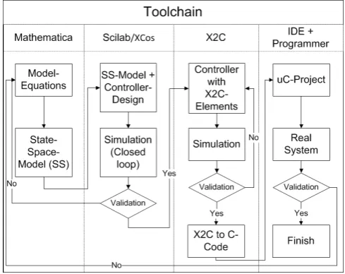
The main idea presented in this paper is the MBD develop-ment using a complete free (or low-cost if target hardware is included) tool-chain starting from the modeling and control design to the hardware realization using an integrated
devel-Figure 1.MBD and the tool-chain.
opment environment (IDE). Possible fields of application for such a low-cost development tool-chain are teaching courses and companies interested in testing this new technology or dealing with MBD projects of moderate complexity.
Our contribution includes the overall concept of the tool-chain, the interaction between the different free software packages, the know-how relating to prameter identification and adaptive self-tuning control and the implementation on the STM32F4µC board.
This paper is organized as follows. Starting with a short description of the parts of the whole tool-chain we focus on the details of the code-generator itself. Afterwards, an ad-aptive control law for the cart system is derived as a non-trivial application. Finally, the model based design process is demonstrated by the implementation of this controller on a low-cost embedded system board.
2
MBD – the tool-chain
[image:1.595.309.554.274.468.2]tures can be extended via add-ons. For example there exists an add-on called “plotting library” that helps the user to make plots with a similar syntax as in Matlab. All plots in this pa-per are done in Scilab. From an engineering point of view, the out-of-the-box incorporation of the Modelica based Coselica (see [8]) is a valuable tool for designers used for standard electrical and mechanical system blocks. System identifica-tion and simulaidentifica-tion verificaidentifica-tion is done in Scilab-XCos too. At least for more dedicated control laws the system has to be described in mathematical terms, i.e., in the form of ODEs. Usually, this is achieved in Mathematica, Maxima or Sage via the Lagrange formalism. Most systems allow the export of equations in a Matlab or C like syntax that can be included into XCos without effort. Of course, these ODEs can be used as plant model too, alternatively to Coselica.
After the controller has been developed and tested in the simulation environment, it must be converted into C-code and transferred to the target. This process should occur as auto-mated as possible. There are several possibilities to generate C-code from an existing XCos schematic. In order to name a few:
• Gene-Auto, [3]: The Gene-Auto project has created an open-source tool set which converts an application de-scribed in a high-level modeling language like Scicos to C-code. Unfortunately, this tool – apart from a commer-cialized toolbox – only works with the previous version of XCos, called Scicos.
• Real-time Linux as target system, [2]: It is one of the longer known tool-chains, but it supports the outdated Scicos and is not really applicable to small embedded systems, i.e. microcontrollers.
• Scicos-FLEX, [4]: It is somehow a port of [2] for some microcontrollers, but outdated too.
As alternative, we make use of our own generator X2C – see below for a more detailed description. Depending on the tar-get, for ARM Cortex-M devices the free emIDE, see [9], is used. There, a general hardware project with the input-output mapping for the STM32F4-discovery board (approx. 15$) has been implemented that directly includes the generated controller code. In order to transfer the program to the target, a SEGGER JLink-EDU (approx. 50$) is used. Nevertheless, it can be replaced by a free JTAG device, e.g., [10]. Altern-atively, there is ongoing development in order to establish an industrial control system (PLC from Bernecker and Rainer, b&r) as an industrial target.
2.1
The code generator X2C [image:2.595.299.538.52.181.2]The code generator X2C, see [5], was originally developed more than ten years ago at the JK-University Linz, Austria as a Simulink extension generating assembler code for TI-DSPs. Later, the system was extended to generate C-code and to largely comply with MISRA (S2C), see [7]. This long history and the simple effective concept of the code generator system stands for stability of its main kernel.
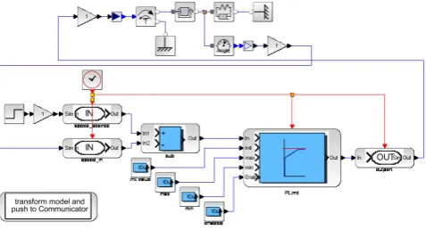
Figure 2.Typical system model with plant (top) and controller (bottom).
X2C natively includes into XCos and can be simulated in parallel with plant and the controller, see Fig. 2. For the plant, blocks of the XCos Coselica library are used. The controller part is modeled using dedicated X2C-XCos blocks. These blocks are full featured XCos blocks extended with an enhanced parameter editor and the connection to the back-end for, e.g., code generation. All the glue code needed for these X2C-XCos blocks is fully auto generated from the X2C block’s model. It is possible and also available to automatic-ally generate blocks for other simulation environments. Spe-cial blocks are used to model and specify the targets in-ports and out-ports which may correspond to, e.g., analog, digital or PWM input or output ports (IOs).
This system model will be simulated to provide detailed feedback about the expected performance of the overall sys-tem for further optimization. In this simulation the blocks im-plement exactly the code which will run on the target. Thus, effects like quantization, fixed point arithmetic artifacts and discretisation are included in the simulation model. In simu-lation the developer has easy access to all signals of the plant and controller to analyse the behaviour or to inject faults for testing.
To move on to the target implementation the model trans-formation and code generation is executed by a single mouse click. The model transformation will step through the XCos model ignoring all non-XCos blocks to detect all X2C-XCos blocks and their associated clock domain and hence the sample time. X2C features the use of multiple sample times for blocks. The result is an abstract model implemented in Java, holding all relevant information about the blocks, their parameters and their connections. Further on, the code gen-erator is applied to this abstract model using methods from graph theory to check, to partition, to order the model and to generate the final code. The generated code is written as substantially MISRA [7] conform ANSI C code in object ori-ented style. During this process the parameters specified in the blocks, usually in the continuous time or frequency do-main, are automatically converted to implementation specific discrete time domain parameters.
During designing the code generator attention has been paid on generation of human friendly, readable code. The generated code facilitates code review, debugging and poten-tial long-term maintenance.
Figure 3.The X2C Communicator with loaded model showing block’s pa-rameter.
Figure 4.X2C Scope: online access to IO ports, block ports, variables and registers of the target.
This operating system features the communication protocol to connect the Communicator, a flash algorithm to deploy the developed control software, to change parameters online, to record data and more. In the case of applying the whole op-erating system, there is no specific target IDE or hardware programmer, besides the target compiler, necessary because the host-target link is established by standard serial (UART, USB) or network connections.
For effective development rapid feedback on changes in design is valuable. With X2C the way from an adapted model to a running system on the target is short even when the whole tool chain of code generator and compiler has to be applied. As a highlight of X2C this is not necessary in many cases. With X2C parameters can be changed in the model or in the Communicator and the parameters on the target are updated instantly. That means manually tuning controller paramet-ers becomes a task of selecting the block and parameter in the XCos diagram and using the keyboard or mouse wheel to tune the parameter while watching the plant and the automat-ically updated Scope for feedback. The Scope, see Fig. 4, is featuring functionality like a conventional oscilloscope. Through the Scope the developer has access to online data of block ports, I/O ports, variables and registers of the target in a way like in the simulation environment.
2.1.1 User defined blocks
[image:3.595.310.555.53.265.2]Own code fragments can be incorporated into simulation and code generation with the help of a dedicated block gen-erator. The user specifies the in- and outputs of the block and
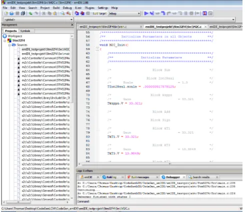
Figure 5.The emIDE with the generated initialization code.
the block generator generates the necessary commented tem-plate files afterwards. The behaviour of the block is included into the templates by the user, and can be used for simula-tion and implementasimula-tion. In the demonstrasimula-tion applicasimula-tion this feature is applied in order to implement a recursive least square algorithm for the adaptive controller.
2.2
emIDE and hardware programmingMost microcontroller developers require full insight into the target programming and a JTAG hardware connection for full on-chip debugging features instead of the small operat-ing system approach already mentioned. Towards this end, we use a free microcontroller IDE, see [9], that supports a vast number of targets. emIDE is a full-featured free em-bedded IDE with stack, register, etc. views and a number of supported JTAG interfaces. In Fig. 5 the initialization part of the heavy commented auto-generated code in emIDE is presented. As soon as standardized names for block IOs in XCos are used only one general template project is required per target, where the hardware specific code parts and espe-cially the input-output mapping take place. As soon as this is achieved for a specific target the user just needs to press the compile and program button. As already mentioned, the small operating system can be used alternatively.
2.3
Different TargetsAs for any other code generator the user acceptance re-lies, among other things, essentially on the number of sup-ported targets. This is the reason why we favor two target ap-proaches, namely the tight integration by the small operating system approach, best fitted for student use, rapid controller prototyping on the real experiments, and the quite versatile approach where all target hardware specific part is done in the IDE. The tight integration approach requires some more target specific details if a new target is made, but releases the user from target hardware interactions. The second IDE-based approach is very easily extendable to new targets.
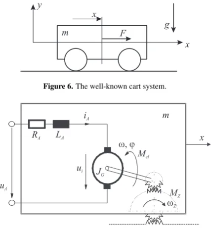
[image:3.595.56.298.245.401.2]Figure 6.The well-known cart system.
R
A LA
u i i A u A M el Q G w, j wZ m z MZ uA
RA LA iA
ui J G
m
x
Mel
Figure 7. Armature equivalent circuit and power conversion of a dc drive with external excitation.
route for the first time, as the feature rich 32bit Flash Cor-texM4 based MCU fits general control purposes very well:
• up to 180 MHz/225 DMIPS, with DSP instructions, floating point unit (FPU; single precision) and advanced peripherals
• 2 DAC 12bit, 3x 12bit ADC (24 channels)
• synchronized PWM-timers, quad-encoder channels • available discovery-board (approx. 15$)
Towards industrial targets (Programmable Logic Controller, PLC) there is ongoing development concerning the applica-tion to a b&r Powerpanel (PP400) using the IDE approach with the target specific Automation Studio.
3
Application: cart system
As a reference application the well-known cart system is presented, see Fig. 6. As common to real world applica-tions the vehicle load capacity is not known. We assume the vehicle massm˜1, linear friction coefficientd˜1and static
fric-tion coefficientFCas unknown, but constant. The cart with
massm1is driven by a dc drive with external excitation, see
Fig. 7.
In the following, we assume a very small electrical time constant (τel = LRA
A, with armature inductanceLA and res-istanceRA) compared to the mechanical one. By means of
system reduction, i.e,LA→0, we introduce equivalent
para-meters integrating the whole drive-train (drive constantkm,
inertia JA, transmission ratio n, gear pinion radius r, and
some mechanical dampingd1) into the mathematical model
of the cart. Other essential parameters are explained in Tab 1.
˜
m1=m1+JA
(n
r
)2
˜
d1=d1+
n2k2m
r2R
A
(1)
The model equations for the non-sticking state of the “slightly” nonlinear reduced system are written to
JA moment of inertia of drivetrain
n transmission ratio km radius pinion
r motor constant RA terminal resistance
2 2.5 3 3.5 4 4.5 5
0 −2 2 −1 1 velocity (v) sign(v)
F0*sign(v) − perfect match F0*sign(v) − worst case error caused by discrete−filtering of sign−function
2 2.5 3 3.5 4 4.5 5
0 −0.1 −0.05 0.05 time [s] error
Figure 8.Worst case approximation error forsign(v)forTs= 10 ms.
( ˙ x ˙ v ) = ( v 1 ˜ m1 (
βuA−d˜1v−FCsign(v)
)) (2)
with the abbreviationβ =nkm(rRA)− 1
and the static fric-tion coefficentFC.
For the calculation of the linear state controller the system has to be written in the formx˙ =Ax+bu. We assume that the static friction is ignored because its value will be identi-fied and compensated in all measurements by the well-known approach. ( ˙ x ˙ v ) = ( 0 1
0 −d˜1 ˜ m1 ) · ( 0 β ˜ m1 )
·uA (3)
3.1
Continuous system identification and adaptive con-trol designAs already mentioned, the cart parameters are assumed un-known but constant. For full physical insight into the adap-tion parameters, we do not identify the sampled, but the con-tinuous plant itself.
In order to get rid of the time derivatives the second equa-tion of the linear system model is transformed from the time domain to the frequency domain. For brevity, initial states are assumed equal to zero.
s2m˜1xˆ=βuˆA−d˜1sxˆ−FCsignˆ(v) (4)
[image:4.595.300.535.54.367.2]0 2 4 6 8 10 12 14 16 18 20 0
−0.1
distance [m]
position servo − parameter identification
0 2 4 6 8 10 12 14 16 18 20 0
5
mass [kg]
0 2 4 6 8 10 12 14 16 18 20 0
20 40
time [s]
lin.friction [Ns/m]
0 2 4 6 8 10 12 14 16 18 20 0
5
time [s]
[image:5.595.61.555.50.431.2]static friction [N]
Figure 9.Offline parameter identification with RLS in Scilab-XCos on true measurements.
sign(v)in a reasonable way. We apply the realizable stable filter with free coefficientsαito both sides
F0(s) =
α0
s2+α
1s+α0
(5)
F1(s) =sF0(s) (6)
s2
s2+α
1s+α0
ˆ
xα0m˜1 =
α0
s2+α
1s+α0
ˆ
uAβ+ (7)
− s
s2+α
1s+α0
ˆ
xα0d˜1 −
α0
s2+α
1s+α0
ˆ
sign(v)FC
see [11]. With standard polynomial division one eliminates the non-strictly proper transfer function. Therefore, it is suffi-cient to implement the two filtersF0(s)andF1(s) =sF0(s).
Both filters have a common denominator and can be realized as one dynamical system if applied to the same signal. The inverse Laplace transform leads to one data line of the algeb-raic equation system for identification
(
α0
(
x−α1
α0F1∗x−F0∗x
)
F1∗x F0∗sign(v)
)
· θθ12
θ3
=F0∗uAβ (8)
linear in the unknown parameters θ1 = ˜m1,θ2 = ˜d1 and θ3 = FC, whereby * indicates the convolution operator in
time-domain. For implementation purpose the filters have to be discretized andsign(v)approximated. Towards this end, the velocity forsign(v) is approximated by the backward difference quotient and further thesign-function by a sum of positive and negative discretized unit steps which only causes a quite small error as long as there is no chattering around zero velocity. Additionally, this error vanishes with the arbit-rary filter time constants as depicted in Fig. 8.
The filter on plant input uA is discretized naturally by a
zero-order hold, but the filters applied to the states have to be approximated. A trapezoidal approximation, i.e., the Tustin method, is usually sufficient without requiring an unnatural small sample time compared to system dynamics. The un-known parameters can be estimated using standard recursive
Figure 10.Cart system - Coselica.
0 1 2 3 4 5 6 7 8 9 10 0
−10 10
voltage [V]
ua_measure ua_sim position servo − state control
0 1 2 3 4 5 6 7 8 9 10 0
0.2 0.4
distance [m]
setpoint x_measure x_sim
0 1 2 3 4 5 6 7 8 9 10 0
−1 1
time [s]
velocity [m/s]
[image:5.595.60.297.334.441.2]v_measure v_sim
Figure 11. Comparison of simulation and true experiment with standard state control and known parameters.
least square (RLS) algorithm. For identification results with the RLS algorithm in XCos on true plant measurements the reader is kindly referred to Fig. 9. The parameter drift un-til 8 s is caused by the unequal mechanical behaviour of the laboratory test bench and the drifting mean value of the pos-ition cycles due to the open loop experiment.
For the adaptive self-tuning control (STC) approach the fil-ters and a standard RLS algorithm are implemented in com-bination with a linear state control law parametrized inm˜1
andd˜1.
The necessary X2C-XCos blocks for parameter identific-ation (signal filtering and RLS algorithm) and STC (control law) are coded manually with the help of the block generator.
3.2
Experiment - Cart systemIn order to demonstrate the physical modeling capabilities the Coselica toolbox is used for plant modeling, see Fig. 10. The quality of the overall model compared to the true exper-iment can be seen in Fig. 11 where a standard linear quasi-continuous (Ts= 1 ms) state controller based on fixed
iden-tified parameters is implemented in simulation and real ex-periment. Velocities are obtained by first order derivative ap-proximations.
3.2.1 Adaptive STC Control
0 1 2 3 4 5 6 7 8 9 10 0
voltage [V]
0 1 2 3 4 5 6 7 8 9 10 0
0.5
distance [m]
setpoint−not activ setpoint−activ actual value
0 1 2 3 4 5 6 7 8 9 10 0
−2 2
time [s]
[image:6.595.45.286.49.249.2]velocity [m/s]
Figure 12.STC control measurement (slashed lines means inactive signals).
The first 2 seconds are used for settling the online RLS iden-tificator and the filters as derived above. Then the paramet-rized control lawuA=−k(θ)Txis activated, see Fig. 12.
k= (
−1576.73 ˜m1
0.2594 ˜d1−40.449 ˜m1
)
(9)
4
Conclusion
The presented work is available for free – to a large extent under a BSD licence, see the references [5], [6].
Ongoing development is targeted towards efficient hand-ling of vectorized signal lines, Scilab-code to C-code con-version, more block libraries, industrial targets, IEC 61131-3 code generation (PLC), adaption of the FMI (functional mockup interface) for model exchange with various commer-cial simulators, and some state machine concept. For most parts we plan to again adapt existing free tools.
Acknowledgements
We gratefully acknowledge the support from the Austrian funding agency FFG in the COIN-project ProtoFrame and
REFERENCES
[1] Scilab: Free and Open Source software for numerical compu-tation, Scilab Enterprises, 2012, http://www.scilab.org/.
[2] Roberto Bucher, et al., RTAI-Lab tutorial: Scilab, Comedi, and real-time control, 2006.
[3] Ana-Elena Rugina, et al., Gene-Auto: Automatic Software Code Generation for Real-Time Embedded Systems, DASIA 2008.
[4] Scicos-FLEX code generator,
http://erika.tuxfamily.org/drupal/scilabscicos.html/ .
[5] X2C in Scilab-XCos, 2013,
http://www.mechatronic-simulation.org/ .
[6] 2013, http://www.modelbaseddesign.at/ .
[7] MISRA Consortium, 2013, http://www.misra.org.uk/.
[8] Reusch, 2013, http://www.kybdr.de/software/.
[9] emIDE the free IDE for embedde programming, 2013, http://www.emide.org/ .
[10] Open On-Chip Debugger, a open JTAG interface, 2013, http://openocd.sourceforge.net/ .