On the Convergence of the Dual Pivot Quicksort Process

(1)

http://dx.doi.org/10.4236/ojmsi.2016.41001

On the Convergence of the Dual-Pivot

Quicksort Process

Mahmoud Ragab

1

_{, Beih El-Sayed El-Desouky}

2

_{, Nora Nader}

2

1_{Department of Mathematies, Faculty of Science, Al Azhar University, Cairo, Egypt} 2_{Department of Mathematics, Faculty of Science, Mansoura University, Mansoura, Egypt}

This work is licensed under the Creative Commons Attribution International License (CC BY).

http://creativecommons.org/licenses/by/4.0/

Abstract

Sorting an array of objects such as integers, bytes, floats, etc. is considered as one of the most im-portant problems in Computer Science. Quicksort is an effective and wide studied sorting algo-rithm to sort an array of n distinct elements using a single pivot. Recently, a modified version of the classical Quicksort was chosen as standard sorting algorithm for Oracles Java 7 routine library due to Vladimir Yaroslavskiy. The purpose of this paper is to present the different behavior of the classical Quicksort and the Dual-pivot Quicksort in complexity. In Particular, we discuss the con-vergence of the Dual-pivot Quicksort process by using the contraction method. Moreover we show the distribution of the number of comparison done by the duality process converges to a unique fixed point.

Keywords

Randomized Quicksort, Convergence, Dual-Pivot Quicksort Process, Running Time Analysis

1. Introduction

Quicksort is one of the important sorting algorithms. Hoare [1] proposed an algorithm depended on selecting an arbitrary element from the array. This element called a pivot element such that Quicksort algorithm used for parting the arrays into two sub-arrays: those smaller than the pivot and those larger than the pivot [2].

(2)

se-lected pivot. There are many cases to choose the pivot element. The worst-case, the best-case and the average case express the performance of the algorithm. We will discuss some of them and for more details; we refer to Ragab [6] and [7]. The worst-case occurs when the pivot is the smallest (or largest) element at partitioning on array of size n, yielding one empty sub-array, one element (pivot) in the correct place and one sub-array of size

n− 1. So, the two sub-arrays are lopsided so this case is defined by worst case [8]. We found the recursion depth is n− 1 levels and the complexity of Quicksort is O n

( )

2 . The best case occurs when the pivot is in the median at each partition step, i.e. after each partitioning, on array of size n, yielding two sub-arrays of approximately equal size and, the pivot element in the middle position takes n data comparisons [9]. There are various methods to choose a good pivot, like choosing the First element, Last element, and Median-of-three elements (selection three elements, and find the median of these elements), and so on. In this case the Quicksort algorithm selects a pivot by random selection each time. This choice reduces probability that the worst-case ever occurs. The other method, which essential prevents the worst case from ever occurring, picks a pivot as the median of the array each time. When we chose the pivot, we compare all other elements to it and we have n− 1 comparisons to

di-vided the array. The choosing of the pivot didi-vided the array into one sub-array of size 0 and one sub-array of size n− 1, or into a sub-array of size 1 and other one of size n− 2, and so on up to a sub-array of size n− 1 and

one of size 0. We have n possible positions and each one is equality in probability 1/n. Hennequin studied com-parisons for array by using Quicksort with r pivots when r = 2, same comparisons as classic Quicksort in one partitioning. When r > 2, he found the problem is complied. Yaroslavskiy [10] introduced a new implementation of Dual-pivot Quicksort in Java 7’s runtime library. In 2012, Wild and Nabel denoted exact numbers of swaps and comparisons for Yaroslavskiy’s algorithm [10]. In this paper, our aim is to analyze the running time perfor-mance of Dual-pivot Quicksort. The limiting distribution of the normalized number of comparisons required by the Dual-pivot Quicksort algorithm is studied. It is known to be the unique fixed point of a certain distributional transformation T with zero mean and finite variance.

We show that using two pivot elements (or partitioning to three subarrays) is very efficient, particularly on large arrays. We propose the new Dual-pivot Quicksort scheme, faster than the known implementations, which improves this situation (see in [11] and [12]). The implementation of the Dual-pivot Quicksort algorithm has been inspected on different inputs and primitive data types.

The new Quicksort algorithm uses partitioning a source array T

[ ]

g, where g is primitive array which we need to sort it. Such as int, float, byte, char, double, long and short, to three parts defined by two pivot elements

p and q (and therefore, there are pointers A, B, C and left and right indices of the first and last elements respec-tively). The aim of this paper is topresent such a version arising from an algorithm depending on the work in [13]

and [14]. The Dual-pivot Quicksort is explained clearly in [15] and it works as follow: 1) For small arrays (length < 17), use the Insertion sort algorithm [10].

2) Choose two pivot elements p and q. We can get, for example, the first element g left

[ ]

as p and the last element g right

[

]

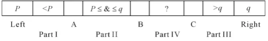
as q.

3) p must be less than q, otherwise they are swapped. So, we have the following parts.

• Part I with indices from left + 1 to A− 1 with elements, which are less than p.

• Part II with indices from A to B− 1 with elements, which are greater or equal to p and less or equal to q.

• Part III with indices from C + 1 to right− 1 with elements greater than q.

• Part IV contains the rest of the elements to be examined with indices from B to C.

4) The next element g B

[ ]

from the part IV is compared with two pivots p and q, and placed to the corres-ponding part I, II, or III.

5) The pointers A, B, and C are changed in the corresponding directions. 6) The steps 4 - 5 are repeated while B≤C.

7) The pivot element p is swapped with the last element from part I, the pivot element q is swapped with the first element from part III.

[image:2.595.181.447.664.705.2]

8) The steps 1 - 7 are repeated recursively for every part I, part II, and part III as in Figure 1.

(3)

2. Run-Time Performance

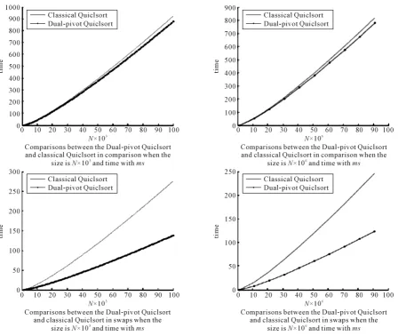
In this section, we introduce some running time of the Dual-pivot Quicksort. An efficient procedure is described by Vasileios Iliopoulos and David B. Penman [13], where they analyzethe Dual pivot Quicksort algorithm. Their approach can be here provided and for more detailswe refer to [13] and [14]. First we introduce the algorithm of it and we compare between it and the classical Quicksort as follows [16].

The following graphs show the relation between the size of array which need to sort and the time of complex-ity which represent by the number of comparisons and swaps as in Figure 2. We found the Dual-pivot Quicksort is faster than classical Quicksort.

3. The Dual-Pivot Quicksort Average Case Analysis

To find the distributional equation, we note the following: for the underlying process, there are two parts. The first part is partitioning and the second is the total number of comparisons to sort an array of n≥2 keys, when the pivot is a uniform random variable

{

1, 2,3,,n

}

is equal to the number of comparisons to sort the sub- array of on

1 1

n

U − keys below the first pivot [17].

In addition, we need to compute the number of comparisons to sort the sub-array of

2

n

n U− elements above the second pivot plus the number of comparisons to sort the sub-array of

2 1 1

n n

U −U − elements between the first and the second pivot.

Plus

1

[image:3.595.93.542.330.708.2]

2n U− _n −2 comparisons done to partition the array which come from when the all elements compare one time with the first pivot and the remain elements compare two times with the second and the first pivot. Therefore,

(4)

1 11 2 2 11

2 2 ,

n n n n

d

n n U n U U U

X = n U− − +X ₋ +X∗₋ +X ₋ ₋ (1)

where the random variables

11

n

U

X ₋ ,

2

n

n U X∗− and

2 11

n n

U U

X ₋ ₋ are identically distributed and independent of

1 n U and 2 n U . Here

d

= refers to the equality in distribution. The array is partitioned into three subarrays one with

1 1

n

U − keys smaller than the first pivot, a subarray of

2 1 1

n n

U −U − keys between two pivots and the part of

2

n

n U− elements greater than the second pivot. The algorithm is then recursively applied to each of these subarrays. The number of comparisons during the first stage is

(

1

) (

2 1

) (

2

)

1 1 2 1 2 ,

n n n n n

A = +_U − + U −U − + n U− _

where

1 1, , 1

n

U =  n− and

2 1 1, ,

n n

U =U +  n. Using [11], the average value of A_n can be calculated as fol-low:

( )

(

) (

)

(

)

₍

₎

1 1 1 1 3 2 1 1 1

1 1 2 1 2

2

1 2 5 7 5 7

2 2 2

1 6 6 3

2 n n

n

i j i

n n

i j i

E A i j i n j

n

n i n n n

n n n

− = = + − = = + = +_ − + − − + − _       −   = − − = _ − + _= −        

∑ ∑

4. Expected Number of Comparisons

Here by Equation (1) and using [13], it is easy to determine the recurrence for the expected number of compari-sons due to the duality as follow:

( )

₍

₎

(

)

(

)

(

)

2

1 1 1

1

1 1 1 1 1 1

5 7 2

1 .

3 1 n

n n n n n n

n i n U j i

i j i i j i i j i

n

E X E X E X E X

n n − − − ∗ − − − = = + = = + = = +   − = + _ − + + _ − 

∑ ∑



Since the three double sums above are equal, then the recurrence becomes

( )

₍

_{) (}

1

) (

)

1 1

5 7 6

, 3 1 n n i i n

E X n i E X

n n − − = − = + − −

∑

setting a_n =E X

( )

_n ,

(

) (

)

1

1 1

5 7 6

, 2. 3 1 n n i i n

a n i a n

n n − − = − = + − ≥ −

∑

By initial conditions we have a₀ =a₁ =0. Multiplying both sides by 2

n

   

 , we obtain

(

) (

)

(

)(

)

(

)

1 1

1 5 7

5 7 6

3 .

2 2 3 1 6

n n

n i i

i i

n n n n n n

a n i a n i a

n n − − − − = =   − −   ₌  − ₊ ₋ ₌ ₊ ₋     _{ } ₋ _    

∑



∑

We introduce a difference operator for the solution of this recurrence. The operator is defined by

( )

:

(

1

)

( )

.

F n F n F n

∆ = ∆ + − (2)

And for higher orders

( )

1

(

)

1

( )

: 1 .

k k k

F n −F n −F n

∆ = ∆ + − ∆

(5)

2 1 1

0

1 5 3

3 .

2 2 2 2

n

n n n i

i

n n n n n

a a a a

− + = +       − ∆_{ } =_ _ −_{ } = +      

∑

1 1

5 1 3 .

2 n 2 n 2 n n

n n n

a + a₊ a n a

     

∆_{ } = ∆_ _ − ∆_{ } = + +      

By definition (2),

2

1 2 1

2 .

2 n 2 n 2 n 2 n 2 n 2 n

n n n n n n

a + a ₊ a + a ₊ + a₊ a

            ∆ _{ } = ∆_ _ − ∆_{ } =_ _ − _ _ +_{ }            

(

n+1

)(

n+2

)

an+2−2n n

(

+1

)

an+1+n n

(

−1

)

an=2 5

(

n+ +1 3an

)

then

(

n+1

) (

(

n+2

)

an+2−

(

n−2

)

an+1

)

+

(

n+2

) (

(

n+1

)

an+1−

(

n−3

)

an

)

=2 5

(

n+1 .

)

Dividing by

(

n+1

)(

n+2

)

, we obtain the telescoping recurrence

(

)

(

)

(

)

(

)

(

)

(

)(

)

2 1 1

2 2 1 3 2 5 1

,

2 1 1 2

n n n n

n a n a n a n a n

n n n n

+ + + + − − + − − + = + + + + + which yields

(

)

(

)

(

)(

)

2 1 1 0

2 2 5 1 18

2 10 18 .

2 1 2 2

n

n n

n j

n a n a j

H n

n j j n

+ +

+ =

+ − − ₌ + ₌ ₊ ₋

+

∑

+ + +

Multiplying by

(

1

)(

2

)(

3

)

24

n− n− n−

, this recurrence is transformed to a telescoping one

(

)(

)

1 1

1 18 1 2 3

10 18

4 n 4 n 24 4 n 4

n n n n n n n

a − a₋ − − − H ₋

        = + + −                

(

)(

)

1

1 1 1

1 2 3

18 10 18 .

4 24 4 4

n n n

n j

j j j

n j j j j j

a H ₋

= = =

− − −

  ₌ ₊   ₋  

     

 

∑

 

∑

  (3)

By using maple V. Iliopoulos and D. B. Penman [13] get

(

)(

)

1

1 2 3 6 .

4

n

j

n

j j j

=

  − − − _{=  }  

∑

And for the other sums in Equation (3):

1 1

.

4 5 5

n

j n

j

j n

H H ₊

= +   ₌  ₋     _ _    

∑

Therefore,

(

)(

)

1

1 1 1 1

1

1 1

4 4 4 4

1 1 1

1 2 3

5 5 24

1 1 1

.

5 5 4 4

n n n n

j j j

j j j j

n

j

n

j j j j

H H H

j j

n

H j j j

n n H − = = = = + = +          = − = −                    +    =_ _ − _− − − −     +      =_ __ − _−_{ }      

∑

(6)

1

1 1

9 1 1

10 18

4 n 2 4 5 n 5 4 4 5

n n n n n

a  + H ₊  +

  ₌  ₊   ₋ ₋  ₋  

 

     _ _               

1

9 1 1 1 1

10 18 .

2 5 5 4 5

n n

a = +  +_ _H₊ − _− _− +

 

 

Finally, the expected number of comparisons, when two pivots are chosen is

(

)

( )

2 1 4 ~ 2 log ,

n n

a = n+ H − n n n (4)

where H_n is the harmonic number defined by

1 1 : n n k H k =

=

∑

(see [18] and [19]).

This is the same value of the expected number of comparisons, when one pivot chosen in the classical Quick-sort [20]. Note that this result for the dual Quicksort is identical with theexpected number of comparisons in

[13].

5. Varience of Comparisons

The main result of this section was obtained by [13] (see following results for explanationand notation). Now we compute the variance of the number of comparisons by Dual-pivot Quicksort. Recall that

( )

5 7

2 2 and .

3

n n

n

A = n− −i E A = − (5)

From Equation (1), we have

(

)

1

(

)

1 1 1 1 1 , 2 n n

n n i j i n j

i j i

P X t P A X X X t

n − ∗ − − − − = = + = = + + + =      

∑ ∑

noting that the resulting subarrays are independently sorted, then we get

(

)

1

(

1

)

(

1

)

(

)

1 1 ,

1

2 2 .

2 n n

n i j i n j

i j i l m

P X t P X l P X m P X t m l n i

n − ∗ − − − − = = +   = = _ = = = − − − + + _      

∑ ∑ ∑

Letting

( )

(

)

0 , t n n t

f z P X t z

∞

=

∑

=

be the ordinary probability generating function for the number of comparisons needed to sort n keys, we obtain

( )

1

( )

2 2 1 1 1 1 1 2 n n n i

n i j i n j

i j i

f z z f z f z f z

n − − − − − − − = = + =      

∑ ∑

(6)

It holds that f_n

( )

1 =1 and f_n′′

( ) (

1 =2 n+1

)

H_n−4n. Moreover, the second order derivative of Equation (6) evaluated at z=1 is recursively given by

( )

₍

₎

(

)

(

)

(

) (

)

(

)

(

)

(

)

(

)

(

)

(

)

(

)

(

)

1 1 1

2

1

1 1 1 1 1 1

1 1

1

1 1 1 1

1 1

1 1 1

1 1 1 1 1

2

2 2 2 2 2 2 2

1

2 2 2 2 2 2

2 2 2

n n n n n n

n i

i j i i j i i j i

n n n n

j i n j

i j i i j i

n n n n n

i j i i n j

i j i i j i i

f z n i n i n i E X

n n

n i E X n i E X

E X E X E X E X

− − − − = = + = = + = = + − − − − − = = + = = + − − − − − − − − = = + = = + =  ′′ = _ − − − − − + − − −  + − − + − − + + +

∑ ∑

(

) (

)

( )

1 1 1

1 1

1 1 1 1 1 1

1 1 1 .

n

j i n j

j i

n n n n n n

i i j n j

i j i i j i i j i

E X E X

f f f

(7)

By simple manipulation of indices, the sums of the products of expected values are equal. The double sum of the product of the mean number of comparisons can be simplified as follows:

(

)

(

)

(

)

( )

(

)

( )

(

)

1 1 1

1 1

1 1 1 0

2 1

1 1

1 5

2 1 4 1 2 .

2 2

n n n n i

i n j i j

i j i i j

n

i i

E X E X E X E X

n i n i n i

i H i

− − − − − − − = = + = = − − = =  _ _{− +} _ _{− −} ₋  = _ + − −  _ _ _+       

∑ ∑

∑

We find

(

)

(

)

(

)

(

)(

)

(

)

1 1 1 1 1 1 1 1 1 1 1 1 1 1 1 1 1 1 1 1 1 1 2 2 1 2 2 1 . n n

i n i i n i

i i

n n

i n i i n i

i i

n n

i n i i n i

i i

n i n i

i H H i H H

n i n i

i H H H H

i n i H H n i H H

− − − − − − = = − − − − − − = = − − − − − − = = − + − +     = − +         − −     = − _ _ + _ _     + − − + −

∑

The recurrence becomes

( )

(

)(

)

(

( )

)

(

) (

) ( )

2 2 2 1 2 1 1 17 47

1 2 1 2 6

3 3

209 731 13 6

1 ,

36 36 6 1

n n n n

n

i i

f n n H H H n n

n n n i f

n n − − =   ′′ = + + − − _ + + _   ′′ + + + + − −

∑

where H_n( )2 is the second order harmonic number defined by ( )2 ₂

1 1 : n n k H k =

=

∑

(see [17] and [18]). Letting

( )

1

n n

d = f′′ and subtracting

2 n

n d

   

  from 1

1 2 n n d₊ +    

  , we get

(

)(

)

(

( )

)

(

)

(

)

2 2 2 2 1 1

4 1 2 84 198 42

2 9

3 79 231 14 .

9

n

n n n

n

i i

n nH

d n n n H H n n

n

d₋ n n

=

 

∆_{ } = + + − − + +  

+

∑

+ + +

By using the identity [4]

( )2 ( )2

2 2 1 1 2 . 1 n

n n n n

H

H H H H

n + − + = − + ₊ 

  (7)

It holds that

(

)(

)

(

( )2

)

(

)

2 ₁₂ ₁ ₂ 2 ₂₀ 2 ₃₂ ₁₂ ₁₇ 2 ₃₇ ₃ _.

2 n n n n n

n

d n n H H H n n n n d

 

∆ _{ } = + + − − + − + + +  

The previous equation is the same as

2 1

2 .

2 n 2 n 2 n

n n n

d ₊ d ₊ d

+ +

     

− +

           

And our recurrence becomes

(

)(

)

(

)

(

)

(

)(

)

(

( )

(

)

(

2 2 2 1 2 2

)

1 2 2 1 1

2 12 1 2 20 32 12 17 37 3 .

n n n

n n n n

n n d n n d n n d

n n H H H n n n n d

+ +

+ + − + + −

(8)

Dividing by

(

n+1

)(

n+2

)

, we obtain the telescoping recurrence

(

)

(

)

(

)

(

)

(

( )

)

(

)

(

)(

)

(

)(

)

2 1 2 ₂ 2 1 2 1 1 2 2 2

20 32 12

1 3 17 37

2 12 .

1 1 2 1 2

n n

n

n n

n d n d

n

H n n

n d n d n n

H H

n n n n n

+ + + + + + − − +  ₊ ₋  + − − _ + _ = + − − +   + _ + + + + _

(

)

(

)

(

)

(

( )

)

(

)

2 1 2

2 2 2 2

1 1 1

2 2

24 100 104 88 292 8 122 346 20,

n n

n n n

n d n d

n n H H H n n n n

+ +

+ + +

+ − −

= + + − − + − + + +

which is equivalent to

(

)

(

)

(

( )

)

(

)

1

2

2 2 2 2

1 4

24 4 88 60 8 122 142 20.

n n

n n n

nd n d

n n H H H n n n n

−

− −

= + − − − − + − +

Again as before, multiplying both sides by

(

1

)(

2

)(

3

)

24

n− n− n−

, the recurrence telescopes with solution

( )

(

)

2

(

2 ( )2

)

₍

₎₍

₎

2

1 1 1

1 4 1 4 1 4 3 23 33 12.

n n n n

f′′ = n+ H ₊ −H₊ − H ₊ n+ n+ + n + n+

Using the well known fact that

( )

(

( )

)

2

1 1 1 ,

n n n n

Var C = f′′ + f′ − f′

the variance of the number of key comparisons of the Dual-pivot Quicksort is (see [17] [19] and [20])

(

)

2 ( )2

₍

₎

2

7n −4 n+1 H_n −2 n+1 H_n+13 ,n

where H_n( )2 is the second order harmonic number defined by (see [18] and[19])

( )2 2 1 1 . n n k H k = =

∑

6. Asympototic Distribution

In this section, we show the convergence results which are essential for the main purpose. Defining a random variables

( )

: , 1

d

n n

n

X E X

Y n

n −

= ≥ (8)

Equation (8) can be rewritten in the following form

( )

(

1 1 1 2 2 1 1

)

1

: 2 2 ,

n n n n

d

n n U n U U U n

Y n U X X X E X

n ∗ − − − − = − − + + + − and so,

(

)

₍

₎

(

)

₍

₎

(

)

₍

₎

(

) (

)

( )

1 1 2 2

1 2

2 1 2 1

2 1 1

2 1

1 2 2 1

1 1 1 1 1 1 1 1 1 1

1 2 2

.

n n n n

n n

n n n n

U U n U n U

n n n

n n

U U U U

n n n

U U

U n U U U n

X E X X E X

Y U n U

n U n U

X E X

U U n U

E X E X E X E X

(9)

By a simple manipulation, one gets

(

)

1 2 2 1

1 1 2

11 2 2 1

1 1

, ,

n n Un Un

n n n n

n U n U n n n

U n U U U

Y Y Y Y C U U

n n − − n

∗ − − − − − −       = _ _+ _ _+ _ _+      

where the cost function

(

)

1, 2

n n n

C U U is given as and it seems to be like in [6] and [7], and given by

( )

(

1

)

(

) (

1

)

( )

)

2 2 1

, = .

n i n j j i n

n i

C i j E X E X E X E X

n n

∗

− − − −

− − ₊ ₊ ₊ ₋

(10)

Now, we show the random vector Un1_,Un2

n n

   

  converges to a uniformly distributed random vector

(

U U1, 2

)

on

[ ]

0,1 . So,

(

)

1 2

, , .

n n D

U U U U n n   →    

  (11)

Here

(

U U₁, ₂

)

is uniformly distributed random vector on

[ ]

0,1 . The moment generating function of

(

Un1,Un2

)

is given by

(

)

(

)

(

)

(

)

( )

( ) ( )

(

)

( ) ( )

11 22

1 2 1 2

1 2 1

1 2

1 1 2 2

1 2

1 1 2 2

1 2

1

1 2 1 2

1

1 2

1 1

2 ₁ ₁

, , e , ,

1 e e 1 e e

e 1 e 1

2 2

2 e e e

.

1 e 1 e 1

k k

n Un

n n

s s

n n n n

k k k

U

s n s s n s

s s

s n s s n s

s s

M U U s s P U U K K

M s M s

n n e n n + − = + + + + +   = _ = _ = − − = − −               − − = _ _ − − −  

∑ ∑

For the random vector Un1_,Un2

n n      ,

(

)

₍ ₎ ( ) ( ) ( ) ( )

(

)

( ) 1

1 2 1 2 2

1 1 2 2

1 2 1

1 1 2 2

1 2

1

1 2 1 2

1 2 _,

,

1

1 1 1 1

2 1 , , 1 1 e e 2 2

1 e e 1 e e

e 1 e 1

2 2

2 e

1

n U

n n n n U n

U U U U

n n

s k s k

n n

k k k

s n n s n s n n s n

s s

s n n

s s s s

M s s M M M

n n n n

n n n n n n         − = + + + + + + +       = _ _= _{ }⋅ _{ }       = ⋅             − − = − −               = _ ₋ _  

∑

( ) 1 2( ) ( ) 2

1 2

1 1 1

e e e

.

e 1 e 1

s n n

s n s n

s s

+ +

− −

Now, the random vector

(

U U₁, ₂

)

has the following moment generating function

( )

(

)

1 2

1 1 2 2 1 1 2 2

1 2

1 1 1 1

1 2 1 2 1 2

,

1 2

0 0 0 0

e 1 e 1

, e d d e d e d .

s s

s t s t s t s t

U U

M s s t t t t

s s

+  −  − 

= = _{= } _ _

  

(10)

By the above Equation (12) the moment generating function of Un1

n is an approximation to the average

val-ue of _es x1 _{over the interval}

[ ]

_0,1 _{. The moment generating function of} Un2

n is an approximation to the

aver-age value of _es x2 _{over the interval}

[ ]

_0,1 _(see_[8]_and_[9]_).

For the cost function

( )

(

1

)

(

) (

1

)

( )

2 2 1

, .

n i n j j i n

n i

C i j E X E X E X E X

n n

∗

− − − −

− − _ _

= + _ + + − _

By using asymptotically, the expected complexity of Dual-pivot Quicksort is 2 logn n given in Equation (4), it follows that

(

) (

)

( )

(

)

(

)

(

)

(

)

1 2

1

1 2 2 1

1 1 2

1 2

2 1

1 1

lim ,

2 2 ₁

lim

2 1

lim 2 2 1 log 1 2 log

2 1 log 1

n n n n

n n

n

U n U U U n

n

n n n

n n

n

n n

U U

C n n

n n

n U

E X E X E X E X

n n

U n U n U

U n n U

n n n n n

n U n U

U U

n n

→∞

∗

− − − −

→∞

 

⋅ ⋅

 

 

− −

 

= _ + + + − _

 

    ⋅   ⋅  =  − − + _  −  − +  −  −

      



⋅ ⋅

 

+ _ − − _ − − −

 

( )

( ) (

) (

)

[ ]

1 1 2 2 2 1 2 1 1 2

2 log

2 2 log 2 1 log 1 2 log , , 0,1 .

n n

ε ε ε ε ε ε ε ε ε ε

 

 _ 

= + + − − + − − ∀ ∈

Thus n1_, n2

n

U U

C n n

n n

 

⋅ ⋅

 

  converges to some C U U

(

1, 2

)

, defined as

(

1, 2

)

2 2 1log

( ) (

1 2 1 2

) (

log 1 2

) (

2 2 1

) (

log 2 1

)

,

C U U = + U U + −U −U + U −U U −U

where U1 and U2 are uniformly distributed random variables on

[ ]

0,1 . Therefore, if we assume for moment that

Yn converges in distribution to some Y, we obtain

( )

(

1

(

1 2

)

(

2 1

)

(

1, 2

)

.

L Y =L YU +Y∗ −U +Y U −U +C U U

Here U U Y Y₁, ₂, , and Y∗ are independent. Y∗ and Y have the same distribution as Y. Finally we show that Y_n converges in fact to the fixed point Y.

Let D be the space of distribution functions F with finite second moments

∫

x F x2d

( )

< ∞ and the first moment

∫

x F xd

( )

=0. We use the Wasserstein metric [4] on D.

(

,

)

inf ₂,

d F G = X −Y

where

2

. denotes the L₂ norm. Defining a map T D: →D by

( )

(

1

(

1 2

)

(

2 1

)

(

1, 2

)

,

T F =L τ X + −τ X∗+X τ −τ +C τ τ

where X X, ∗,X,

τ

₁ and τ₂ are independent .

( )

.

L X =L X∗ =L X =F

Here τ1 and τ2 are uniformly distributed random variables on

[ ]

0,1 and C is a map defined as C: 0,1

[ ]

→.

We have to refer to Roesler (see in [4] [21] and [22]) for the main idea for the next lemma.

Lemma 1

(11)

( )

2

( )

, , , , ,

F T F T F  F∈D converges in the d-metric to fixed point of T.

Proof

Let F and G are in D

( )

(

1

(

1 2

)

(

2 1

)

(

1, 2

)

.

T F =L τ X + −τ X∗+X τ −τ +C τ τ

( )

(

1

(

1 2

)

(

2 1

)

(

1, 2

)

.

T G =L τY+ −τ Y∗+ τ −τ Y +C τ τ

( )

.

L X =L X∗ =L X =F

( )

.

L Y =L Y∗ =L Y =G

The random variables

τ τ

₁, ₂,X X, ∗ and X are independent. Also

τ τ

₁, ₂, ,Y Y∗ and Y are independent. Here τ₁ and τ₂ are uniformly distributed on

[ ]

0,1 . Then

( ) ( )

(

)

(

)

(

)

(

)

(

)

(

)

(

)

(

) (

)

(

)

(

)

(

)

(

)

(

)

( )

(

)

(

)

(

)

(

)

(

)

(

)

(

)

(

)

(

)

(

)

2

1 2 2 1 1 2 1 2 2 1 1 2 ₂

2

1 2 2 1

2

2 2

2 2 2 2

1 2 2 1

2 2

2

,

1 , 1 ,

1

1 1 1

3 3 6

5

, 6

d S F S G

X X X C Y Y Y C

X Y X Y X Y

E X Y E E X Y E E X Y E

E X Y E X Y E X Y

E X Y

τ τ τ τ τ τ τ τ τ τ τ τ

τ τ τ τ

∗

∗ ∗

≤ + − + − + − − − − − − ≤ − + − − + − −

≤ − + − − + − −

 

≤ _ − + − + − _

 

≤ −

where

( )

3 1

1

2 2 1

1 ₀1 1 0

1

d .

3 3

E τ = τ τ = _{ }τ =

 

∫

(

)

(

)

(

)

(

)

1 3 1

2 2 2

2 ₀ 2 2

0

1 1

1 1 d .

3 3

E τ τ τ τ

 ₋ 

− = − − = −  =

 

 

∫

(

)

(

)

(

)

(

)

( )

( ) ( )

1 1 1 1

2 2 ₂ ₂

1 2 _{0 0} 1 2 1 2 _{0 0} 1 1 2 2 1 2

1 1

3 2

1

1 ₂ 1 ₂

1 1

2 2 1 2 2 2 2

0 0 0

0 0

1

2 3

2 2

2

0

d d 2 d d

1 1

2 d 2 d

3 2 3 2

1 1 1 1

.

3 2 3 3 2 3 6

E

t

τ τ τ τ τ τ τ τ τ τ τ τ

τ _τ τ _{τ τ} _τ _τ _τ _τ

τ τ

τ

− = − = − +

  _ _

 

= − ⋅ + ⋅ = _ − ⋅ ⋅ + _

   

 

 

 

= − + = − + =

 

 

∫ ∫

∫

Taking the infimum over all possible

(

X Y,

)

we obtain

( ) ( )

(

)

5

(

)

, , ,

6

d T F T G ≤ d F G

using Banach fixed point theorem completes the proof (also see[13]).

Acknowledgments

(12)

References

[1] Hoare, C.A.R. (1962) Quicksort. The Computer Journal, 5, 10-15. http://dx.doi.org/10.1093/comjnl/5.1.10

[2] Rosler, U. (2001) On the Analysis of Stochastic Divide and Conquer Algorithms. Algorithmica, 29, 238-261. http://dx.doi.org/10.1007/BF02679621

[3] Regnier, M. (1989) A Limiting Distribution for Quicksort. Informatique Théorique et Applications, 23, 335-343.

[4] Roesler, U. (1992) A Fixed Point Theorem for Distributions. Stochastic Processes and their Applications, 42, 195-214. http://dx.doi.org/10.1016/0304-4149(92)90035-O

[5] Roesler, U. and Rueschendorf, L. (2001) The Contraction Method for Recursive Algorithms. Algorithmica, 29, 3-33. http://dx.doi.org/10.1007/BF02679611

[6] Ragab, M. (2011) Partial Quicksort and Weighted Branching Processes. PhD Thesis, 28-35.

[7] Ragab, M. and Rosler, U. (2014) The Quicksort Process. Stochastic Processes and their Applications, 124, 1036-1054. http://dx.doi.org/10.1016/j.spa.2013.09.014

[8] Fill, J.A. and Janson, S. (2001) Approximating the Limiting Quicksort Distribution. Random Structures Algorithms, 19, 376-406. http://dx.doi.org/10.1002/rsa.10007

[9] Fill, J.A. and Janson, S. (2004) The Number of Bit Comparisons Used by Quicksort: An Average-Case Analysis. ACM-SIAM Symposium on Discrete Algorithms., New York, 300-307 (Electronic).

[10] (2009) http://permalink.gmane.org/gmane.comp.java.openjdk.core-libs.devel/2628

[11] Ragab, M. (2015) Partial Quicksort and Weighted Branching Process: Surveys and Analysis. LAP Lambert Academic Publishing, Germany.

[12] Fuchs, M. (2013) A Note on the Quicksort Asymptotics. Random Structures and Algorithms.

[13] Iliopoulos, V. and Penman, D.P. (2012) Dual Pivot Quicksort. Discrete Mathematics, Algorithms and Applications, 04, No. 3. http://dx.doi.org/10.1142/S1793830912500413

[14] Iliopoulos, V. (2013) The Quicksort Algorithm and Related Topics. PhD Thesis. Department of Mathematical Sciences, University of Essex. http://repository.essex.ac.uk/13266

[15] Martinez, C., Nebel, M.E. and Wild, S. (2014) Analysis of Branch Misses in Quicksort. SIAM. http://dx.doi.org/10.1137/1.9781611973761.11

[16] Wild, S., Nebel, M.E. and Martienz, C. (2014) Analysis of Pivot Sampling in Dual-Pivot Quicksort. arXiv preprint ar-Xiv:1412.0193.

[17] Wild, S. (2012) Java 7’s Dual Pivot Quicksort. Master Thesis, University of Kaiserslautern, Kaiserslautern, Germany. http://www.uni-kl.de/en/home/

[18] Choi, J. and Srivastava, H.M. (2011) Some Summation Formulas involving Harmonic Numbers and Generalized Har-monic Numbers. Mathematical and Computer Modelling, 54, 2220-2234.

http://dx.doi.org/10.1016/j.mcm.2011.05.032

[19] Wild, S., Nebel, M.E., Reitzig, R. and Laube, U. (2013) Engineering Java 7’s Dual Pivot Quicksort. Proceedings of the ALENEX 2013, New Orleans, Louisiana, USA, 7 January 2013, 55-69.

[20] Wild, S. and Nebel, M.E. (2012) Average Case Analysis of Java 7’s Dual Pivot Quicksort . In: Epstein, L. and Ferra-gina, P., Eds., Algorithms—ESA 2012, Springer, Berlin/Heidelberg, 825-836.

http://dx.doi.org/10.1007/978-3-642-33090-2_71

[21] Wild, S., Nebel, M.E. and Mahmoud, M. (2014) Analysis of Quickselect Under Yaroslavskiy’s Dual-Pivoting Algo-rithm. Algorithmica, 78, 485-506. http://dx.doi.org/10.1007/s00453-014-9953-x

[22] Wild, S., Nebel, M.E. and Neininger, R. (2013) Average Case and Distributional Analysis of Java 7’s Dual Pivot Quicksort. arXiv preprint arXiv:1304.0988.

(13)

Appendix

A1. The Dual-Pivot Quicksort Algorithm [15]

DUALITY -PIVOT QUICKSORT (G, left, right) // Sort G left

[

,,right

]

(including end points).

1) If right – left < M // i.e. the sub-array has n ≤ M elements 2) INSERTIONSORT (G, left, right)

3) Else

4) If G left

[ ]

>G right

[

]

5) p:=G right

[

]

; q:=G left

[ ]

6) Else

7) p:=G left

[ ]

; q:=G right

[

]

8) End If

9) A:=left+1; B:=right−1; B:=A

10) While B≤C

11) If G B

[ ]

<p

12) Swap G B

[ ]

and G A

[ ]

13) A:= +A 1

14) Else 15) If G B

[ ]

≥q

16) While A C

[ ]

>q and B<C do C:= −C 1 End While 17) If G C

[ ]

≥ p

18) Swap G B

[ ]

and G C

[ ]

19) Else

20) Swap G B

[ ]

and G B

[ ]

; Swap G B

[ ]

and G A

[ ]

21) A:= +A 1

22) End if 23) C:= −C 1

24) End if 25) End if 26) B:= +B 1

27) End While

28) A:= −A 1; C:= +C 1

29) G left

[ ]

:=G L

[ ]

; G L

[ ]

:=p // Swap pivots to final position 30) G right

[

]

:=G C

[ ]

; G C

[ ]

:=q

31) DUALITY-PIVOT QUICKSORT

(

G left L, , −1

)

32) DUALITY-PIVOT QUICKSORT

(

G L, +1,g−1

)

33) DUALIY-PIVOT QUICKSORT

(

G g, +1,right

)

34) End if

A2. The Implementation of the New Dual-Pivot

Here’s the implementation of the new Dual-Pivot (Yaroslavskiy) in java: public main void sort(double[] g) {

sort(g, 0, g.length); }

public main void sort(double[] g, double fromIndex, double toIndex) { rangeCheck(g.length, fromIndex, toIndex);

Yaroslavskiy(g, fromIndex, toIndex - 1, 3); }

private main void rangeCheck(double length, double fromIndex, double toIndex) { if (fromIndex > toIndex) {

(14)

}

if (fromIndex < 0) {

throw new ArrayIndexOutOfBoundsException(fromIndex); }

if (toIndex > length) {

throw new ArrayIndexOutOfBoundsException(toIndex); }

}

private main void swap(double[] g, double i, double j) { int tem = g[i];

g[i] = g[j]; g[j] = tem; }

private static void dualPivotQuicksort(double [] g, double left, double right, double div) { double lenth = right - left;

if (lenth < 27) { // insertion sort for tiny array for (double i = left + 1; i <= right; i++) { for (int j = i; j > left &&g[j] < g[j - 1]; j--) { swap(g, j, j - 1);

} } return; }

int third = len / div; // "medians" int s1 = left + third; int s2 = right - third; if (s1 <= left) { s1 = left + 1; }

if (s2 >= right) { s2 = right - 1; }

if (g[s1] < g[s2]) { swap(g, s1, left); swap(g, s2, right); }

else {

swap(g, s1, right); swap(g, s2, left); }

// chosse the pivots double first pivot =g[left]; double second pivot = g[right]; // pointers

double less = left + 1; double great = right - 1;

// sorting the array by the Dual pivot Quicksort for (int k = less; k <= great; k++) {

if (g[k] < first pivot) { swap(g, k, less++); }

(15)

until (k > great && g[great] < second pivot) { great--;

}

swap(g, k, great--); if (g[k] < first pivot) { swap(g, k, less++); }

} } // swaps

double Dis = great - less; if (Dis < 13) {

div++; }

swap(g, less - 1, left); swap(g, great + 1, right);

// recursive the algorithm for the arrays Yaroslavskiy(g, left, less - 2, div); Yaroslavskiy(g, great + 2, right, div); // subarray

if ( first pivot < second pivot) { Yaroslavskiy(g, less, great, div); }