Design of Hard and Soft Decision Decoding Algorithms of LDPC

Design of Hard and Soft Decision Decoding

Algorithms of LDPC

Namrata P. Bhavsar

Computer Engineering Department, Parul Institute of Engineering & Technology,

Limda, Waghodiya, Vadodara.

Brijesh Vala

Asst. Prof. Computer Engineering Department, Parul Institute of Engineering & Technology,

Limda, Waghodiya, Vadodara.

ABSTRACT

The demand for satellite communication and a wide-ranging objective, however, is often to achieve maximum data transfer, in a minimum bandwidth while maintaining an satisfactory quality of transmission. The transmission quality is basically concerned with the probability of bit error at the receiver here with respect to communication. This is an attempt to achieve highest capacity with minimum error rate by implementing modern codes named as LDPC(Low Density Parity Check codes) and it is represented here various decoding schema to decode and encode them At the present time LDPC codes has received a superior interest because their error correction performance and their functional world wide applications. The paper represents LDPC significance ,its characteristics and encoding and iterative decoding approaches to achieve channel capacity. Thus we need some technology that utilizes this available bandwidth by providing good error correction capability. We can also achieve it by using FPGA spartan 3e’s VHLD implementation.

General Terms

Iterative decoding, LDPC, encoding.

Keywords

Bit Error Rate, Tanner graph, parity check codes, Bit Flipping, Sum Product Algorithm.

1. INTRODUCTION

LDPC was introduced by Robert Gallager at MIT in 1960 in his PhD thesis[1].Low density parity check codes are linear block codes using generator matrix G in an encoder and parity check matrix H in a decoder[1]. The parity check matrix has M rows and N columns, where M represents check nodes and N represents variable nodes. Here the matrix is based on random construction techniques. Information bits depends on check nodes and code word bits are depends on variable nodes. Tanner Graph is the bipartite graph introduced to graphically represent these codes. They also helps to describe decoding algorithms. Tanner graphs are separated into two distinctive sets and edges are only connecting nodes of two different types mainly known as check nodes and variable nodes. The iterative decoding of code is the true optimum decoding if tanner graph contains no cycles. Therefore we want LDPC codes with few cycles. Low-density parity-check (LDPC) codes are a class of linear block codes[4]. The name comes from the characteristic of their parity-check matrix which contains only a few 1’s in comparison to the amount of 0’s.The advantage is that they provide a performance which is very close to the capacity for a lot of different Channels and linear time complex algorithms for decoding [2].

1.1 LDPC Codes : Construction

LDPC Codes are Special Linear block codes with sparse parity-check matrix H with dimensions M × N. To denote the length of code N and K to denote its dimension with information bits M=N-K. Hi,j =1 if code bit i is involved in the parity check equation j , and otherwise 0.Here all the operations are carried out in binary field. Since generally the parity check matrices are not in the symmetric form, symbol A is used to represent the parity check matrices and H for parity check matrices in symmetric form. The generator matrix G is N*K and parity check matrix A is (N-K)*N such that H.G=0 .m is message vector of size k*1 and code word vector of size c*1.The row of parity check matrix as

A = 𝑎1𝑇

𝑎_.2𝑇

. 𝑎𝑀𝑇

The equation 𝑎𝑖𝑇𝑐 = 0 is said to be linear parity check

construction on code word c. The notation Zm=𝑎𝑚𝑇 c.

where Zm is parity check[2] . The generator matrix for

encoding purpose corresponding to the parity check matrix A is as per following. Using Gaussian elimination with column pivoting as necessary to determine an M*M matrix 𝐴𝑝−1 so that

H =𝐴𝑝−1𝐴 =[I A2]

Here H from

G= 𝐴2

𝐼

while A may be sparse, neither the systematic generator G nor H is necessarily sparse. A matrix is said to be sparse if fewer than half of the elements are nonzero.

1.2 Representation of LDPC Codes

Any linear code has a bipartite graph and a parity-check matrix representation. The matrix bellow is a parity check matrix with dimension n × m for a (8, 4) code. We have defined two numbers describing the matrix.Here Wr for the number of 1’s in each row and Wc for the columns. For a matrix to be called low-density the two conditions Wc< =n

H =

0 1 0

1 1 1 1 1 0 0 10 0 1 0 0 0 0 1

[image:2.595.94.241.72.118.2]

1 0 0 0 0 1 1 11 1 0 1 0

Fig 1: Matrix Representation (LDPC) [4]

The sparse property of LDPC gives rise to its algorithmic advantages. An LDPC code is of two types: Regular and irregular. It issaid to be regular if Wc is constant for every column and Wr is constant for every row & Wr = Wc

𝑛 𝑚 . If

Wc is constant for every column and is also constant for every row, then the LDPC code is said to be regular. The example matrix is regular with Wc = 2 and Wr = 4.Through the graphical representation, we can also see the regularity of LDPC codes. There is the same number of incoming edges for every v-node and also for all the c-nodes. If H is low density but the numbers of 1’s in each row or column aren’t constant the code is called a irregular LDPC code.

Tanner in 1981 introduced an effective graphical representation for LDPC Tanner codes. Not only provide these graphs a complete representation of the code, they also help to describe the decoding algorithm. The two types of nodes ina Tanner graph are known here as variable nodes (v-nodes) and check nodes(c-(v-nodes) Tanner graph is also called as bipartite graph. The reason behind it is that the nodes of the graph are separated into two distinctive sets and edges are only connecting nodes of two different types.

Fig 2: Tanner Graph corresponding to parity check matrix of 8 column (N) and 4 row(M)[4]

The tanner graph consists of m check nodes i.e. the number of parity bits and n variable nodes i.e. the number of bits in a codeword. And here Check node fi is connected to variable

node cj if the element hij of H is a 1.

1.3 Encoding of LDPC Code

Encoding of codes, specially of who has higher block lengths can be quite difficult to implement in hardware but there are several methods of generating H such that encoding can be done via shift registers. If the generator matrix G of a linear block code is known then encoding can be done using Parity check matrix[2].The cost of the method depends on the Hamming weights i.e. the no of 1’s of the basis vectors of G. If the vectors are dense, then cost of encoding using this method is proportional to n2[9].If G is sparse then this cost becomes linear with n. However here if the LDPC is given by the null space of a sparse parity-check matrix H, It is unlikely that the generator matrix G will also be sparse. So one of the straightforward method of encoding LDPC that would require number of operations which is proportional to n2. As this is too slow for most practical applications, It is desirable to have encoding that run in linear time. Here note that by performing Gauss-Jordan elimination on H to obtain it in the form a

generator matrix G for a code with parity-check matrix H which can be found as per following.

H= 𝐴 𝐼𝑛−𝑘

Where A is (n-k)×k binary matrix and 𝐼𝑛−𝑘 is the size n-k

identity matrix. The generator matrix is then

G= 𝐼_𝐾 𝐴𝑇

Now at here we can encode this message into code words for LDPC Codes which requires the generation of parity check matrix H[2]. The encoding method is through the use of a generator matrix, denoted by G. A code word c is formed by multiplying source message u by the matrix which is represented as c=u*G. The constraints which are recognized from matrix G are contained by parity check equations of the LDPC code. For a binary code if it is given that if there are k message bits and length of the codeword is n, then the generator matrix G is a (k *n) binary matrix will be in the form =_𝐴𝑇𝐼𝐾. As the row space of G will be orthogonal to H,here GHT = 0. The process of converting H into the generator matrix G has the effect of causing G to lose the sparseness characteristic that was embodied in H.

Orientation of paper

Section I contains basic terms for LDPC code and requirements for efficient decoding algorithms. Literature survey is in Section II. Section III contains Hard and soft decoding schemas and their significance for decoding LDPC codes. Section IV contains overview of FPGA spartan 3E platform. Finally in Section V indicates conclusion is i.e to increase data rate.

2. HARD DECISION DECODING

There are different iterative decoding algorithms having two derivations. They are mainly classified as in hard decision decoding and soft decision decoding respectively. There are various algorithms to deal with decoding of LDPC codes. They are classified according to their complexities to get decoded for different codes. First of all here in this hard decoding scheme the check nodes finds the bit in error by checking the parity which may be even or odd and the messages from variable nodes are transmitted to check nodes, check node checks the parity of the data stream received from variable nodes connected to it. And then If number of 1‘s received at check nodes satisfies the required parity, then it sends the same data back to message node, else it adjusts each bit in the received data stream to satisfy the required parity and then transmits the new message back to message nodes. So here in case each node fj looks at the message received

from the variable nodes and calculates the bit that the fourth variable node should have n order to fulfil the parity check equation[3].The bit flipping algorithm is an example of hard decision decoding. The bit flipping decoder is going to be immediately terminated, whenever a valid code word has been found. By checking if all the parity check equations are satisfied then it the process get terminated.

f

0

f

1

f

2

f

3

[image:2.595.49.278.382.505.2]

2.1 Bit flipping Algorithm

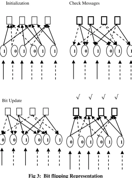
[image:3.595.317.558.70.195.2]

A binary hard decision about the each received bit is made by detector and passed to another decoder. Here in the bit-flipping algorithm the messages passed along the Tanner graph edges and a bit node sends a message declaring if it is a one or a zero, and then each check node sends a message to each connected bit node by finally declaring that what value the bit is based on the information available to the check node. The check node at this step finds that if the modulo-2 sum of the incoming bit values is zero, its parity-check equation is satisfied. The bit node changes (flips) its current value, if the majority of the messages received by a bit node are different from its received value[4]. This process of algorithm is repeated which is known as iteration and it is repeated until, some maximum number of decoder iterations has passed and the decoder gives up or until all of the parity-check equations are get satisfied. Thus how the bit flipping algorithm is known as hard decision decoding algorithm.

Fig 3: Bit flipping Representation

[image:3.595.318.547.248.383.2]

In bit flipping in the first step the following circuit is required to XOR the input message bits at variable nodes each time to check parity check equations at check nodes. As per Specified in figure 4. Another figure circuit is required to check for whether to flip the bit or not to get the correct word. As shown in figure 5 , inputs are given to gates by considering 0 as no complement and 1 as complement to receive output.

Fig 4 : XOR circuit to check parity at check nodes

Now in step 2 it is required to flip the bit which is incorrect and following circuit would help to flip the bits.

Fig 5 : Circuit to flip the bits

3. SOFT DECISION DECODING

Soft-decision decoding gives enhanced performance in decoding procedure of LDPC codes which is based on the idea of belief propagate. In soft scheme, the messages are the conditional probability that in the given received vector received bit is a 1 or a 0. The sum-product algorithm is a soft decision message-passing algorithm. Priori probabilities for the received bits is the input probabilities as here they were known in advance before running the LDPC decoder. The bit probabilities returned by the decoder are called the a posterior probabilities[3].

3.1 Sum Product Message Passing

Algorithm (SPA)

The sum-product algorithm is a soft decision message-passing algorithm which is similar to the bit-flipping algorithm described in the previous section, but the major difference is that the messages representing each decision with probabilities in SPA. Whereas bit-flipping decoding on the received bits as input, accepts an initial hard decision and the sum-product algorithm is a soft decision algorithm which accepts the probability of each received bit as input[3].For example here initially take a guess that suppose a binary variable x, then it is easy to find P(x = 1) given P(x = 0), since P(x = 1) = 1−P(x = 0) and so here it is needed to store one probability value for x. Log likelihood ratios are introduced here to do so. They are used to represent the metrics for a binary variable by a single value as per following:

L(x) = Log(

𝑃(𝑋=0)

𝑃 𝑋=1

)

Initialization

0 1 0 1 1 1

Check Messages

Bit Update

Test

0 1 0 1 1 0

√ √ √ √

1 0 1 0 1 1

[image:3.595.51.284.271.584.2]

The aim of sum-product decoding algorithm here is first to compute the maximum a posteriori probability (MAP) for each codeword bit. Now here it is the probability that the i-th codeword bit is a 1 conditional on the event N and that all parity-check constraints are satisfied. The sum-product algorithm iteratively computes an approximation of the MAP value for each code bit. The a posteriori probabilities returned by the sum-product decoder are only exact MAP probabilities if the Tanner graph is cycle free[3].The extra information about bit i received from the parity-checks is called as extrinsic information for bit i. Until the original a priori probability is returned back to bit i via a cycle in the Tanner graph, the extrinsic information obtained from a parity check constraint in the first iteration is independent of the a priori probability information for that bit and information provided to bit i in subsequent iterations which remains independent of the original a priori probability for bit i. In sum-product decoding the extrinsic message from check node j to bit node i, Ej,i, is the LLR of the probability that bit i causes parity-check j to be satisfied[3].

The probability that the parity-check equation is satisfied if bit i is a 1 is,

𝑃

_{𝑗 ,𝑖}𝑒𝑥𝑡

=

1

2

-

1

2

𝛱

𝑖′∈𝐵𝑗 ,𝑖′≠𝑖

(1-2

𝑃

𝑖′

𝑖𝑛𝑡

_{) ………….(1)}

Where 𝑃𝑗 .𝑖𝑒𝑥𝑡 is the current estimate, available to check j, of the

probability that bit i‘ is a one. If bit i is a zero, The probability that the parity-check equation is satisfied is thus (1 - 𝑃𝑗 ,𝑖𝑒𝑥𝑡).

Here it is expressed as a log-likelihood ratio,

𝐸

𝑗 .𝑖

= LLR(

𝑃

𝑗 ,𝑖𝑒𝑥𝑡

) = log(

1−𝑃_{𝑗 ,𝑖}𝑒𝑥𝑡

𝑃_{𝑗 ,𝑖}𝑒𝑥𝑡

)………….(2)

And substituting (2) we get

E

i

,

j

= log(

1+ 𝛱𝑖∈𝐵𝑗 ,𝑖′≠𝑖tan ℎ(

𝑀 𝑗 ,𝑖′

2 )

1− 𝛱𝑖∈𝐵𝑗 ,𝑖′≠𝑖tan ℎ(

𝑀 𝑗 ,𝑖′

2 )

)……..(3)

Where

M

j

,

i’

= LLR(

𝑃

𝑗 ,𝑖𝑖𝑛𝑡_′

) = log(

1−𝑃_{𝑗 ,𝑖′}𝑖𝑛𝑡

𝑃_{𝑗 ,𝑖′}𝑖𝑛𝑡

)

Here Each bit has access to the input a priori LLR, ri, and the LLRs from every connected check node. The total LLR of the i-th bit is the sum of these LLRs:

𝐿

_𝑖

= LLR(

𝑃

_𝑖𝑖𝑛𝑡

) = r

i +

∑

𝑗 ∈𝐴_𝑖

𝐸

𝑗 .𝑖 ………..

(4)

The messages sent from the bit nodes to the check nodes, Mj,i, are not the full LLR value for each bit here. The equation Hx[mod 2] = 0 is satisfied (where x[mod 2] is received codeword) or maximum number of iterations set.

4. THEORITICAL COMPARISON and

ANALYSIS

This paper’s aim here is to reach the most efficient approach to increase BER for satisfying the most demanding parameter of data rate by achieving highest channel capacity. The decoding algorithms named bit flipping is having hard decision characteristic of probabilities and Sum Product Algorithm is having Soft decision making characteristics for probabilities of messages. As described in the previous section, SPA issimilar to the bit-flipping algorithm but with the messages representing each decision with probabilities.In contrast to taht bit-flipping decoding accepts an initial hard decision on the received bits as input, the sum-product algorithm is a soft decision algorithm which accepts the probability of each received bit as input[7].The Represented simulation Results of these algorithms on MATLAB are here.

[image:4.595.308.558.296.507.2]

The simulation parameters here for bit flipping are SNR is 0 to 15,BER is 10^-2 and M=500 ,N=1000.

Fig 6: Iterative Decoding of Bit flipping

Expected Result of SPA:

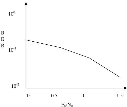
The SPA algorithm increases the BER rate to increase the channel capacity as it is a soft decoding iterative algorithm. The simulation results for expected outcomes are as follows in figure 7 where -1=10−1.

0 0.5 1 1.5

10-2 10-1 100

Eb/N0

[image:5.595.86.516.74.356.2]

Fig 7: Error performance for iterative decoding of the (1008, 504) LDPC code with SPA concept

5. OVERVIEW OF FPGA SPARTAN 3E

PLATFORM

Implementing MATLAB code here involves feature of the above kit like Converting floating-point MATLAB code to fixed-point MATLAB code with optimized bit widths which is suitable for efficient hardware generation. Identifying and mapping procedural constructs to concurrent area- and speed-optimized hardware operations. Then after introducing the concept of time by adding clocks and clock rates to schedule the operations in hardware and creating resource-shared architectures to implement expensive operators like multipliers and for-loop bodies. The following kit diagram represented here with its logic gates and external ports and Display.

Fig 8: FPGA SPARTAN 3E kit[8]

Feature of kit involves Very low cost, ,LVCMOS, LVTTL, HSTL, and SSTL single-ended signal standards& 622+ Mb/s data transfer rate per I/O, Enhanced Double Data Rate (DDR) support ,DDR SDRAM support up to 333 Mb/s, flexible logic resources, Efficient wide multiplexers, wide logic ,Fast look-ahead carry logic ,Enhanced 18 x 18 multipliers with optional pipeline ,Frequency synthesis, multiplication, division, high-performance logic solution for high-volume consumer-oriented applications Multi-voltage, multi-standard Select IO interface pins ,Up to 376 I/O pins or 156 differential signal pairs etc [8].

6. CONCLUSION

[image:5.595.60.275.574.716.2]

7. ACKNOWLEDGEMENTS

A whole heartedly thank to Mr. Brijesh Vala for all his diligence, guidance, encouragement, inspiration and motivation throughout and to thanks to anonymous reviewers for their valuable suggestions.

8. REFERENCES

[1] R. G. Gallager, ‘Low-Density Parity-Check Codes’. Cambridge, MA: M.I.T. Press, 1963.

[2] Analysis and implementation of soft decision decoding algorithm of ldpc, m. M. Jadhav, ankit pancholi, dr. A. M. Sapkal asst. Professor, e&tc, scoe, pune university phase-i, d,-402, g.v 7, ambegaon, pune (india),[IJETT],2013.

[3] Iterative Decoding schemes of LDPC codes, Ashish Patil, Sushil Sonavane, Prof. D. P. Rathod / International Journal of Engineering Research and Applications (IJERA), March -April 2013.

[4] LDPC Codes – a brief Tutorial,Bernhard M.J. Leiner, Stud.ID.: 53418L [email protected],April 8, 2005.

[5] Introducing Low-Density Parity-Check, Codes,Sarah J. Johnson, School of Electrical Engineering and Computer Science, The University of Newcastle, Australia.

[6] Systematic construction, verification and

implementation methodology for LDPC codes

[7] Hui Yu*, Jing Cui, Yixiang Wang and Yibin Yang,Springer.

[8] An introduction to LDPC codes, William E Ryan, department of electrical and computer engineering. The University of Arizona,Australia,2003.

[9] Spartan-3E Starter Kit Board User Guide ,UG230 (v1.0) March 9, 2006