Comparison between Wind Farm Aggregation
Techniques to Analyze Power System Dynamics
Ahmed M. Atallah,
Ph.DElect. Power & Machine Dept., Faculty of Eng. Ain-Shames Univ., Cairo, Egypt
Mona A. Bayoumi
Elect. Power & Machine Dept., Faculty of Eng. Ain-Shames Univ., Cairo, Egypt
ABSTRACT
With increasing amount of wind power penetration, wind farms begin to influence the power systems. When a power system with many wind turbines is to be simulated, Wind farm aggregation techniques are required to reduce the model order while maintaining its accuracy. Different wind farm techniques have been proposed to simulate and analysis wind farm dynamics. In this paper a comparison between three famous techniques: 1- full aggregated model using equivalent wind speed; 2- full aggregated model using average wind speed; and 3- semi aggregated model. Simulation have been carried out for these techniques and compare them using different effects such as wind farm power, reactive power and system dynamics, besides the effect of varying variance on these techniques.
Keywords
Wind farm aggregation, dynamic wind farm model, wind speed variance and doubly fed induction generators.
1.
INTRODUCTION
Wind energy is increasing its contribution to energy generation worldwide. its capacity has reached 159.213 GW (2% of global electricity consumption) worldwide with a growth rate of 31.7% in 2009. By the year 2020 a foreseeable penetration of 12% of global electricity demand (1900 GW) is predicted [1]. With the increasing amount of wind power penetration in power systems; wind farms begin to influence power systems. So it requires adequate models for wind farms to represent overall power system dynamic behavior for grid connected wind farms.
There are different wind turbine generators types are currently widely applied in wind power today. The main comparison can be made between fixed speed and variable speed wind generator concepts. The directly grid coupled squirrel cage induction generator, used in fixed speed wind turbines. The two variable speed wind generator concepts are the doubly fed induction generator and the converter driven synchronous generator [1]. Doubly fed induction generators (DFIGS) wind turbines are largely deployed in wind farms [2] due to their advantages such as: the variable speed generation, the decoupled control of active and reactive powers, the reduction of mechanical stresses, less noise, improvement of power quality, and use of smaller power converter (rated power of only 25% of total wind system power).
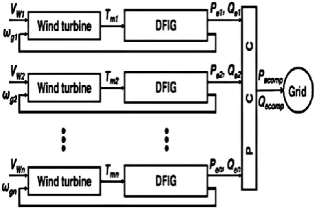
A wind farm contains a large number of individual wind turbine generators, possibly exceeding 100 of wind turbines. Modeling each of these wind turbine generators separately increases the complexity and compromises the simulation speed significantly. A complete wind farm model with n number of wind turbines equipped with doubly fed induction generator (DFIG) is shown in Fig. 1. The complete wind farm model can be simplified by using an aggregated wind farm
[image:1.595.316.539.273.424.2]model, the data requirement and the simulation computation time. This aggregated model can first represent the behavior (active and reactive power exchanged with the grid) during normal operation, characterized by small deviations and the changes of wind speed. Secondly it represents the behavior of wind farm during grid disturbances, such as voltage drops and frequency deviations [3].
Fig. 1. Block diagram of a complete DFIG wind farm model.
In this paper we have chosen three techniques and compared them between the complete model as a reference. These techniques are:
1- Full aggregated model using average wind speed technique [3].
2- Full aggregated model using equivalent wind speed method (EWM) [4].
3- Semi aggregated model [5].
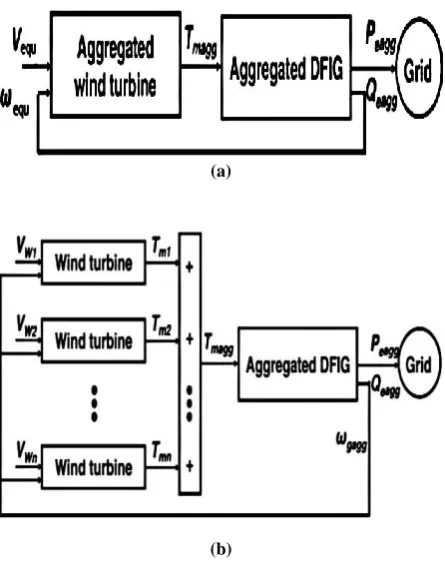
is aggregated and the resulting torque is applied to an equivalent generator system as shown in Fig. 2(b).
(a)
[image:2.595.314.541.66.494.2](b)
Fig. 2. Block diagram of (a) full aggregated and (b) semi aggregated DFIG wind farm models.
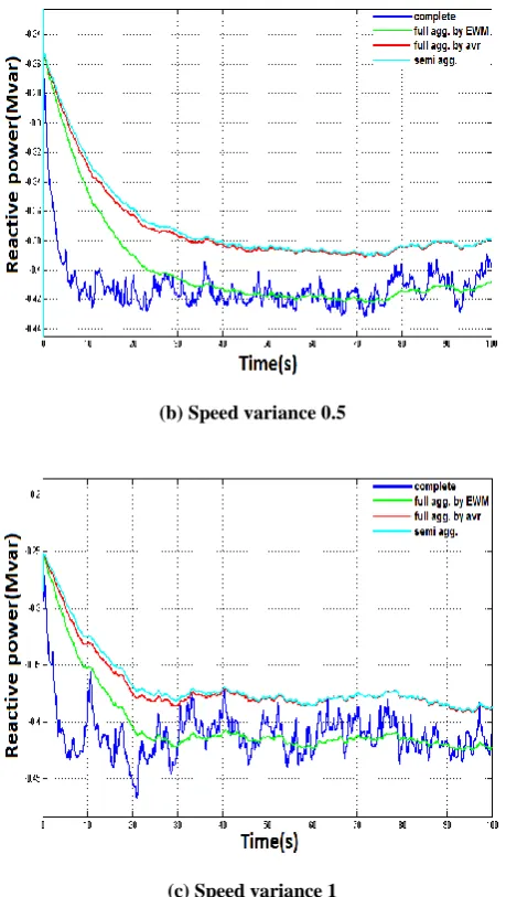
Also we have compared the active power using these techniques for different speed variances (speed variances are 0.1, 0.5, and 1) where the whole wind farm have the same variance in each case as shown in Fig. 3(a,b,c). We can conclude that the effect of variance on the closeness of any aggregated method to the complete solution can not be seen. The same results are found in Fig. 4(a,b,c) when comparing reactive powers.
(a) Speed variance 0.1
(b) Speed variance 0.5
(c) Speed variance 1
Fig. 3. Active power with different variance speed
[image:2.595.56.279.94.376.2]
(b) Speed variance 0.5
[image:3.595.52.282.69.476.2](c) Speed variance 1
Fig. 4. Reactive power with different variance speed
2.
COMPLETE WIND FARM MODEL
[image:3.595.318.541.221.407.2]As shown in Fig. 5 a DFIG wind farm contains a large number of DFIG wind turbines operating at an internal electrical network (lines and transformers) which enables the generated power to be delivered to grid. A complete model represents dynamic response of a DFIG wind farm, in which all the wind turbines and internal electrical network are modeled.
Fig. 5. DFIG wind farm.
2.1
DFIG Wind Turbine
The basic configuration of a DFIG wind turbine is depicted in Fig. 6. The most significant feature of this kind of wound-rotor machine is that it has to be fed from both stator and wound-rotor side. Normally, the stator is directly connected to the grid and the rotor is interfaced through a variable frequency power converter. This power converter made of two back to back IGBT bridges based voltage source converters linked by a DC bus. It decouples the electrical grid frequency and the mechanical rotor frequency, thus enabling variable speed wind turbine generation. In high wind speeds, the power extracted from the wind can be limited by pitching the rotor blades. [1].
Fig. 6. DFIG wind turbine.
The DFIG wind turbine has been represented by modeling the rotor, drive train, induction generator, power converter and the protection system. The parameters of the DFIG wind turbine used in this paper are shown in Table 1 [9].
Table 1. DFIG wind turbine parameters.
Parameter Symbol Value Unit Nominal mechanical output
power
Pmec 1.5 MW
Nominal electrical power Pe 1.5/.9 MW
Nominal voltage (L-L) Vnom 575 V
Stator resistance Rs 0.00706 p.u.
Stator leakage inductance Ls 0.171 p.u.
Rotor resistance Rr 0.0058 p.u.
Rotor leakage inductance Lr 0.156 p.u.
Magnetizing inductance Lm 2.9 p.u.
Base frequency f 60 Hz
Inertia constant H 0.84 s
Friction factor F 3 p.u.
Pair of poles p 0.01 -
2.1.1
Rotor model
The wind power Pw captured by the wind turbine is given by [1].
,
5
.
0
3
wC
(1)where Pw(W) is the aerodynamic power, ρ(kg/m 3
[image:3.595.315.543.484.658.2] [image:3.595.56.279.596.735.2]v(m/s) the wind speed, and Cp the turbine coefficient of
performance which is a function of the tip speed ratio λ (ratio between blade tip speed and wind speed) and θ the pitch angle of rotor blades. The power extracted from the wind is maximized if the rotor speed is such that Cp is maximum,
which occurs for a determined tip speed ratio.
2.1.2
Drive train model
The drive train of DFIG wind turbine has been represented in this paper by the two masses model [1]:
dt
d
r r m wt
2
(3)
dt
D
m r g m r gm
(4)dt
d
g g g m
2
(5)where Twt & Tm are the mechanical torque from the wind
turbine rotor shaft and from the generator shaft, Tg is the
generator electrical torque, Hr & Hg are the rotor and
generator inertia, Km and Dm are the stiffness and damping of
the mechanical coupling.
2.1.3
Generator model
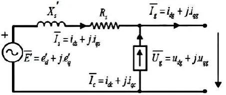
[image:4.595.55.282.379.475.2]Basically, DFIG is an induction type generator. The equivalent circuit of DFIG is shown in Fig. 7.
Fig. 7. Equivalent circuit of DFIG wind turbine.
The wound rotor induction generator has been represented by the third-order model for stability transient studies of power systems. This model is obtained by neglecting the stator transients for the fifth order model of induction generator. It presents three differential equations [6]: two are electrical equations and the third equation is mechanical, given by (5). The model is expressed into a direct and quadrature reference frame rotating at synchronous speed with the position of the direct axis aligned with the maximum of the stator flux. It enables the decoupled control of active and reactive powers of DFIG [7]. Equations (6-9) are electrical differential expressed per unit and use generator convention, which means that the currents are positive when flowing towards the grid.
qr m r m s q s qs s s d d
u
L
L
L
e
s
i
e
T
dt
de
1
(6) dr m r m s d s ds s s q qu
L
L
L
e
s
i
e
dt
de
1
(7)
dsqr qsdr
m
g
L
i
i
i
i
(8)where u denotes voltage, i denotes current, indexes d and q, the direct and quadrature components, indexes s and r refers to stator and rotor, e'd and e'q are the internal voltage
components of induction generator, ɷs is the synchronous
speed, s is the generator slip, T'o is the transient open circuit
time constant, Tg is the generator electrical torque, Xs is the
stator reactance and X's is the transient reactance, expressed as
m r m s s s m s s s m m rL
L
L
L
L
L
L
L
2,
,
(9)with Rs and Rr are the stator and rotor resistances,
L
sandL
rthe stator and rotor leakage inductances and Lm the
magnetizing inductance.
The bidirectional converter is composed of two back to back IGBT bridges linked by a DC bus. A converter is connected to the rotor winding (rotor side converter) and the other converter to the grid (supply side converter) [8]. The rotor side converter controller aims to control the DFIG active power output for tracking the input power of the wind turbine, and maintains the terminal voltage to the reference value. The active power and voltage are controlled independently via uqr
and udr, respectively. The grid side converter controller aims
to maintain the DC link voltage, and control the terminal reactive power [7].
2.1.4. Control system
The control of DFIG wind turbine is consist of three controllers: rotor speed, blade pitch angle and reactive power controller as shown in Fig. 8(a,b,c). The control of wind turbine is based on the following control strategies [8]:
1. Power optimization below rated wind speed. In this case, the wind turbine generates the optimum power corresponding to the maximum power coefficient. The blade pitch angle controller keeps the pitch angle to its optimal, whereas the tip speed ratio is driven to its optimal value by the rotor speed controller acting on the rotor speed/generator torque.
[image:4.595.314.539.563.720.2]2. Power limitation above rated wind speed. The wind turbine operates with the power limited to the rated value. In this case, the rotor speed controller assures the rated power by acting on the rotor voltage, whereas the blade pitch angle keeps the generator speed limited to the control value by acting on the pitch angle.
Fig. 8. Controllers of a DFIG wind turbine: (a) rotor speed controller, (b) reactive power controller and (c) blade
2.1.4
Protection system
Protection system is used to protect the electronic devices used in the power converter by limiting the rotor voltage and current. DFIG wind turbine presents a crowbar [7], which protects the rotor and power converter against over-current. It is external rotor impedance, coupled via the slip-rings to the generator rotor instead of the converter. When a grid disturbance occurs and the control system detects a rotor current value above the current protection limit, the rotor side converter is disabled and bypassed by the crowbar protection. In this case, DFIG is turned into squirrel cage induction generator, and the independent controllability of active and reactive power gets lost.
2.2 Wind Farm Electrical Network
The wind farm electrical network is modeled by the static model of electric lines and transformers, represented by constant impedance, as usual for power systems simulations [6].
A matlab simulation has been done to present the proposed systems.
3.
POWER CURVE OF DFIG WIND
TURBINE
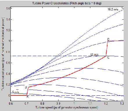
[image:5.595.318.539.86.214.2]The power curve of the DFIG wind turbine model from SimPowerSystems is shown in Fig. 9 [9]. Each point on the power curve represent three values, turbine output power, wind speed, and turbine speed. By the ABCD curve, from zero speed to speed of point A the mechanical power of the DFIG is zero. Between point A and point B the curve is introduced to smooth the power fluctuations occurring near point A.Between point B and point C, DFIG uses the optimal tracking strategy (OPTS) to capture maximum wind energy during the incoming wind speed which is less than the nominal wind speed (NWS). When incoming wind is greater than NWS, the blade pitch control is used to reduce the mechanical power to the equipment rating, which corresponds to the horizontal line starting from D. Between point C and point D the curve is introduced to smooth the power fluctuations occurring near NWS.
Fig. 9. Power curve of DFIG from SimPowerSystems
Table 2 shows the data regarding the four points A-D of the power curve.
Table 2. Data of point A-D
Points Wind speed (m/s)
Turbine speed (p.u.)
Turbine output power
(p.u.)
A 4.23 0.7 0
B 7.1 0.71 0.151
C 12 1.2 0.73
D 13.48 1.21 1
4.
EQUIVALENT WIND METHOD
(EWM)
The EWM from [10] is used for the aggregation of DFIG wind turbines. This equivalent wind is derived from the power curve of the wind turbine, according to the following procedure:
1. The output power of each wind turbine Pj is derived from
its power curve corresponding to the incoming wind.
j wt wtj
C
(10)where PCwt(vj) is a function which represents the power curve
of the wind turbine against wind speed and the super index wt represents the value in p.u., expressed in the individual wind turbine base.
2. The equivalent power Peq is the sum of the output power of
all wind turbines power,
nj wt j wt
eq
1
(11)
3. After that,
eqwtis expressed in the equivalent wind turbinebase as
eqewt. Where the resulting power curve expressed in the equivalent wind turbine base is the same as the individual wind turbines,
eq ewt ewteq
C
(12)wt
ewt
C
C
(13)4. The equivalent wind speed of the whole aggregated system is derived from the inverse function of the power curve.
ewt eq ewteq
C
1
(14)5. If all aggregated DFIG wind turbines faced above nominal winds, the equivalent wind is the average wind speed.
5.
SIMULATION RESULTS
[image:5.595.54.275.501.693.2]Fig. 10. A 9 MW wind farm connected to a distributed system
The complete, full aggregated and semi aggregated model are simulated using Matlab software to obtain the dynamic responses at the PCC under the following two conditions: 1- normal operation and 2- grid disturbance. The variables considered for the comparison are the active (Pe) and reactive
power (Qe) exchange between the wind farm and power
[image:6.595.59.278.71.269.2]system. Table 3 shows the speed of the wind received by the DFIG wind turbines.
Table 3. Wind speeds incident on the wind turbines
Wind turbine
WT1 WT2 WT3 WT4 WT5 WT6
Wind speed (m/s)
6.9 7.8 8.9 9.4 10.3 11.2
5.1 Normal Operation
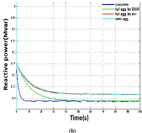
During normal operation, the wind farm operates under wind speed fluctuations. In this case, the wind farm has been simulated with different incoming winds. The collective responses of the complete, two full aggregated and semi aggregated wind farm models at the PCC during normal operation are shown in Fig. 11.
(a)
(b)
Fig. 11. (a) Active power at PCC during normal operation. , (b) Reactive power at PCC during normal operation
The results depicted in Fig. 11(a, b) shows that the full aggregated model using EWM is closer in the results of the complete aggregated model.
5.2 Grid Disturbance
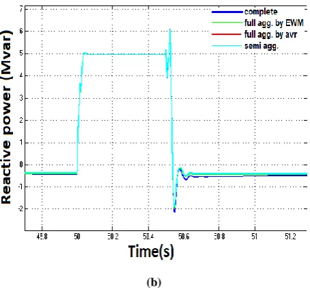
A voltage sag of 50% lasting for 500 ms is originated at the PCC at t = 50 s to evaluate the collective responses of the complete, two full aggregated and semi aggregated wind farm models during grid disturbances at PCC as shown in Fig. 12.
[image:6.595.55.279.544.761.2](b)
Fig. 12. (a) Active power at PCC during grid disturbance. , (b) Reactive power at PCC during grid disturbance
From Fig. 12(a,b) we can conclude that the full aggregated model using EWM is also much closer in the results of the complete aggregated model during the simulation of grid disturbances. This means that we can relay on full aggregated model using EWM even at cases of system dynamic disturbances.
The simulations have been carried out on a personal computer with the following specifications: Intel (R) Core (TM) i5-2430M CPU @ 2.40 GHz 2.40 GHz 2.99 GB of RAM. The computation time takes 103, 89, and 85 second for full aggregated using EWM, full aggregated using average wind speed, and semi aggregated model compared with 924 second for the complete model. This observation demonstrates that any of the three techniques consume lesser time than the complete model for only 6 wind turbines.
6.
DISCUSS THE RESULTS
The results depicted in Figs. 11, 12 shows that the full aggregated model using EWM has a higher correspondence in approximating active and reactive power to the complete model during normal operation and grid disturbance. Unlike in ref [3] where he proposed aggregation technique with the incorporation of a mechanical torque compensation factor (MTCF) into the full AWF model. They compare between full aggregated model using average wind speed and semi aggregated model. Also ref [5] concluded that semi aggregated model is close to complete model. But they did not use the full aggregated model with the equivalent wind speed which gives the best and closest results to the complete technique with a fast simulation computation time.
7.
CONCLUSION
In this paper, a comparison between complete, two full aggregated and semi aggregated models are simulated using Matlab simulation program. First we examine the effect of varying the variance of the applied wind speeds on different proposed aggregated models and we found that no clear evidence that varying the variance effects differently on different aggregated models. Second the full aggregated model using EWM gives the accurate approximation of the collective responses at the PCC in magnitude with a fast simulation computation time during normal operation and grid disturbance.
8.
REFEERNCE
[1] L.M. Fernández, J. R. Saenz, and F. Jurado, “Aggregated dynamic model for wind farms with doubly fed induction generator wind turbines,” Renewable Energy, vol. 33, pp. 129–140, 2008.
[2] M.I. Martinez, A. Susperregui, G. Tapia, and L. Xu, “Sliding-mode control of a wind turbine-driven double-fed induction generator under non-ideal grid voltages,” Renewable Power Generation, IET, vol. 7, pp. 370 - 379, 2013.
[3] A. Chowdhury, W.X. Shen, N. Hosseinzadeh, and H.R. Pota, “A novel aggregated DFIG wind farm model using mechanical torque compensating factor,” Energy Conversion and Management, vol 67, pp.265–274, 2013 [4] Z. J. Meng, and F. Xue, “Improving the Performance of
the Equivalent Wind Method for the Aggregation of DFIG Wind Turbines,” Power and Energy Society General Meeting, 2011 IEEE, pp. 1-6.
[5] M. A. Chowdhury, N. Hosseinzadeh, M. M. Billah and S. A. Haque, “Dynamic DFIG wind farm model with an aggregation technique,” ICECE 2010, 18-20 December 2010, Dhaka, Bangladesh
[6] Heier S. Grid integration of wind energy conversion systems. Chicester: Wiley; 1998.
[7] Ekanayake JB, Holdsworth L, Wu X, and Jenkins N, “Dynamic modeling of doubly fed induction generator wind turbines,” IEEE Trans Power Syst 2003;18(2): 803–9.
[8] L. M. Fernandez, C. A. Garcia, J. R. Saenz, and F.Jurado, “Equivalent models of wind farms by using aggregated wind turbines and equivalent winds,” Energy Conversion and Management, vol. 50, pp. 691–704, 2009.
[9] SimPowerSystems, User’s guide, Natick, MA: The Mathworks Inc., 2011.
[image:7.595.54.281.71.281.2]