Slope Year for the U Pb Dating Method and Its Applications

http://dx.doi.org/10.4236/ojg.2015.55032

Slope Year for the U-Pb Dating Method and

Its Applications

Jie Yuan

Key Laboratory of Earth and Planetary Physics, Institute of Geology and Geophysics, Chinese Academy of Science, Beijing, China

Email: [email protected]

Received 30 April 2015; accepted 23 May 2015; published 26 May 2015 Copyright © 2015 by author and Scientific Research Publishing Inc.

This work is licensed under the Creative Commons Attribution International License (CC BY). http://creativecommons.org/licenses/by/4.0/

Abstract

The slope year

t

slope

for the U-Pb dating method is given as

(

238 235

)

235238 1

ln

slope

t = k

−

λ

λ λ λ

,

where

λ238 and λ235 are the decay constants for 238U and 235U, respectively, and k is the slope of the tangent

line at a point on either the Concordia or Discordia line. These two lines are determined by the initial 206(7)_{Pbi concentrations in minerals. If} 206_Pb 207_{Pb 0}

i = i = , the line is the Concordia.

How-ever, if 206 207

Pbi≠ ∧0 Pbi =0 (∧ is the logical operator “and”, also known as the logical

conjunc-tion), 206 207

Pbi = ∧0 Pbi ≠0 or

206 207

Pbi≠ ∧0 Pbi ≠0, the line is Discordia. The Concordia line is

of the form 206 238

(

207 235

)

238 235

Pbp Up= Pbp Up+1 −1

λ λ

(where p stands for the present), while the Discordia line has the form 206 238

(

207 235

)

Pbp Up=k× Pbp Up +b (where k and b are the slope and intercept of the straight line, respectively).

Keywords

Slope Year, U-Pb Dating, Zircon, Mass Spectrum, Isotope, Initial Pb Isotope Concentration

1. Introduction

In nature, uranium has three radioactive isotopes: 238U(99.2743%), 235U(0.7200%) and 234U(0.0057%) [1] [2]. The former two isotopes decay in the forms:

238 206 4

92U 82Pb 8 He2 6β Q

−

and 235 207 4

92U 82Pb 7 He2 4β Q

−

→ + + + ,

where Q is the heat, β denotes the beta decay and He stands for the element Helium. The decay constants λ for

238_{U and} 235_{U are}

(

)

10

( )

238 1.55125 0.00672 10 1

λ

_{= ± ×} −

σ

a−1 and

λ

₂₃₅=

(

9.8485 0.00083±

)

×10−10

( )

1

σ

a−1, respectively [2]-[4].

These nuclear reactions occur in host minerals, such as zircon (ZrSiO4), and are the basis of the U-Pb dating method in geology [5]-[8]. In a mineral, Pb and U isotopes obey the exponential decay law:

(

238

)

206 206 238

Pb Pb U e t 1

p i p

λ

= + − (1)

and 207_Pb 207_Pb 235_U

(

_e235t ₁

)

p i p

λ

= + − , (2)

where the subscripts i and p represent the initial measurement time and the present, respectively, and t is the age of the mineral [1] [6].

The coordinates n(206Pbp)/n(238Up) (n, the number of isotopes in the bracket) as the ordinate and n(207Pbp)/ n(235Up) ratios as the abscissa form the Pb/U ratio diagram (Figure 1). Samples formed t years ago plot on either

the Concordia or Discordia lines [9]-[12]. For instance, the classical Discordia line was discovered by Ahrens (1955) in Zimbabwe. Equation (1) divided by 238U_p is n(206Pbp)/n(238Up):

238

206 206

238 238

Pb Pb

e 1

U U

p i t

p p

λ

= + − . (3)

Similarly for n(207Pbp)/n(

235

Up), we have

235

207 207

235 235

Pb Pb

e 1

U U

p i t

p p

λ

= + − , (4)

from Equation (2).

To interpret the Discordia line, conventional theories have proposed: 1) this line was caused by Pb loss or U gain after formation of the host mineral [9] [11]-[17], 2) the upper intersection of the Discordia and Concordia lines represents the crystallization age of the mineral [12] and 3) the lower intersection of the Discordia and Concordia lines represents the metamorphic age of the mineral [14].

However, previous theories are not tenable when used in the following cases: 1) the lower intercept point is negative or

2) no upper intercept point exists.

For instance, in Zheng et al. (2012) (Figure 1), all zircons in YX1 from Yingxian lamproites were found to be discordant and yielded a lower intercept age of −370 ± 690 Ma. According to conventional theories, this age in-dicates that the samples will experience a metamorphic process in a distant age. In addition, in Zheng et al.

(2012), all zircons in HBxa from Hebi basalt are also discordant, but yield no upper intercept age. According to conventional theories, these data indicate that the samples did not crystallize until the present. Apparently, the explanations do not conform to the objective facts: the samples are in front of scientists now. New studies should thus focus on resolving these discrepancies.

Herein, the slope years tslopes for the U-Pb dating method for the Concordia and Discordia lines are presented,

and a method for estimating values for tslope from the experimental data is proposed. In addition, four examples

are presented to illustrate the application of the proposed method.

2. Methodology

2.1. Basic Assumptions

In this study, the basic assumptions for the U-Pb dating method included the following:

a) The decay constants λ238 and λ235 are precisely determined. For instance, the decay constants in Jaffey et al. (1971) are of good quality and widely accepted. The number of citations of this paper is greater than 1200 (data from Web of Science);

[image:3.595.221.515.83.254.2]

Figure 1. Pb/U ratio diagram. This diagram shows the predicament for conventional theories. The Concordia (blue, colour for online version) and classical Discordia (black) for Zimbabwe samples (black diamond points) (Ahrens, 1955) are illus-trated. This Discordia and Concordia intercept at A and B, for which the meanings in conventional theories are shown in the lower-right corner. Two counter-examples to traditional theories are also shown: HBxa (hexagon points and red Discordia, Zheng et al. (2012)) and YX1 (right triangle points and green Discordia, Zheng et al. (2012)). See discussions in text.

c) Present 206(7)Pbp and 235(8)Up isotope concentrations in host minerals can be precisely measured using mass

spectrometry (MS). Such MS instruments include sensitive high mass-resolution ion microprobe (SHRIMP) [46] [47], LaserProbe-inductively coupled plasma mass spectrometry (LP-ICPMS) [48] and Cameca IMS-series [44] [49], etc.

2.2. Slope k and Slope Year Tslope

In mathematics, the variance on the ordinate is a function of the variance on the abscissa [50]. Therefore,

n(206Pbp)/n(238Up) is a function of n(207Pbp)/n(235Up) in the Pb/U diagram (Figure 2):

(

)

206 238 207 235

Pb_p U_p = f Pb_p U_p . (5) The theoretical expressions for this function under different conditions are given in Section 2.4.

Next, the slope k of the tangent line at point A on the general curve of Equation (5) was determined. The par-tial derivative of 206Pbp 238Up (Equation (3)) with respect to t is

238

206

238

238 Pb

U

e

p

p t

t

λ

λ

 

∂ _ _

 _{ =}

∂ . (6)

Similarly, we have

235

207

235

235 Pb

U

e

p

p t

t

λ

λ

 

∂ _ _

 _{ =}

∂ (7)

from Equation (4). Equation (6) divided by Equation (7) gives

(238 235)

206

206 238

238

238

207 207

235

235 235

Pb

Pb U

U

e

Pb Pb

U U

p

p p

p t

p p

p p

t

t

λ λ

λ λ

−

 

∂ _ _{  } ∂

  _ _

 

∂ _{= =}

   

∂_ _ ∂_ _

   

∂

[image:4.595.206.444.88.280.2]

Figure 2. Pb/U ratio diagram. The general curve (in blue) for 206Pb_p 238U_p= f

(

207Pb_p 235U_p

)

and tangent line at point A on this curve are shown. The definition of the slope at this point is also given.

In this equation, the second part is the definition of the slope of the tangent line [50]:

( 238 235)

206

238

238 207

235 235

Pb

U

e Pb

U

p

p t

p

p

k λ λ λ

λ

−

 

∂ _ _

 

= =

 

∂ _ _

 

. (9)

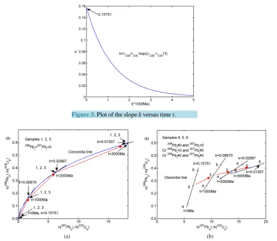
This equation indicates that if t is determined, the value of k is a constant (Table 1) since t ≥ 0, 0 < k ≤0.1575. In addition, the slope monotonically decreases with increasing time t (Figure 3).

If k is determined (see Section 2.6), the slope year is given by rewriting Equation (9):

(

238 235

)

235238 1

ln

slope

t λ k

λ λ λ

=

− . (10)

2.3. Initial

206(7)

_Pb

_i

_{Concentrations in Minerals}

If the values for tslope, 206(7)Pbp and 235(8)Up are known, the initial 206(7)Pbi concentrations in minerals can be

de-termined using the following:

(

238

)

206 206 238

Pb Pb U e tslope 1

i p p

λ

= − − (11)

and 207 207 235

(

235

)

Pb Pb U e tslope 1

i p p

λ

= − − , (12)

which are derived from Equations (1) and (2). Clearly, the concentrations are greater than or equal to zero: ( )

206 7

Pbi ≥0.

2.4. Mathematical Expressions for the Concordia and Discordia Lines

The initial 206(7)Pbi isotope concentrations determine the mathematical expressions for the general graph in

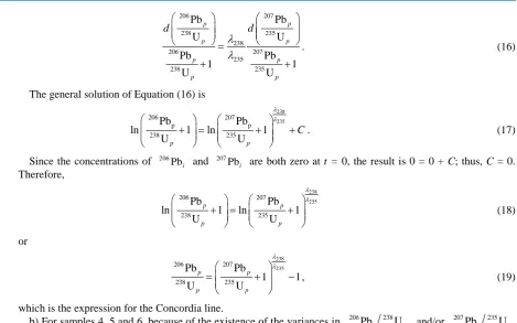
Fig-ure 2. This relationship can be demonstrated using assumed samples formed at the same time t with specific ini-tial conditions. Assume there are three samples (1, 2 and 3,Figure 4(a)) with

206 207

[image:5.595.117.522.81.433.2]

Figure 3. Plot of the slope k versus time t.

[image:5.595.197.409.629.690.2]

(a) (b)

Figure 4.Histories of Pb/U ratios (blue circle) for different samples on (a) Concordia and (b) Discordia. The red arrows in-dicate the direction of the evolution of each ratio.

Table 1. Values of the slope for specific years.

t(Ma) 0 100 1000 2000 3000 4000 5000

ka _{0.15751 0.14497 0.06870 0.02997 0.01307 0.00570 0.00249}

a, calculated from Equation (9)

206 207

206 207

206 207

Or Pb 0 Pb 0

Or Pb 0 Pb 0

Or Pb 0 Pb 0

i i

i i

i i

≠ ∧ =

= ∧ ≠

≠ ∧ ≠

. (14)

The mathematical expressions are given by solving the first-order differential Equation (9) using Equations (3) and (4):

238 235

206 206 206

238 238 238

238 238

207

207 207

235 235

235 235 235

Pb Pb Pb

1

U _e U U

Pb e

Pb Pb

1

U U

U

p p i

t

p p p

t

p

p i

p p

p d

d

λ λ

λ λ

λ λ

 

  − +

 

 _{ = =}

 

− +

 

 

 

. (15).

The solution to this equation is different for each set of samples.

206 207 238 235 238 206 207 235 238 235 Pb Pb U U Pb Pb 1 1 U U p p p p p p p p d d λ λ              ₌   + +

. (16)

The general solution of Equation (16) is

238 235 206 207 p p 238 235 Pb Pb

ln 1 ln 1

Up Up

C λ λ     + = + +        

    . (17)

Since the concentrations of 206_Pb

i and

207_Pb

i are both zero at t = 0, the result is 0 = 0 + C; thus, C = 0.

Therefore, 238 235 206 207 238 235 Pb Pb

ln 1 ln 1

U U p p p p λ λ     + = +        

    (18)

or 238 235 206 207 238 235 Pb Pb 1 1 U U p p p p λ λ   =_ + _ −

  , (19)

which is the expression for the Concordia line.

b) For samples 4, 5 and 6, because of the existence of the variances in 206Pbi 238Up and/or

207 235 Pbi Up

(Equation (14)), Equation (15) is not an elementary function and the solution to it cannot be obtained using ele-mentary integral calculus.

This difficulty can be overcome in the following manner. Consider a geological body (containing samples 4, 5 and 6) with continuous 206Pbi, 207Pbi, 238Ui and

235_U

i distributions. Then

206_Pb 238_U

i i and

207_Pb 235_U

i i

in the system are continuous variables [50]. Looking back to the original differential Equation (9):

206 238 207 235 Pb U Pb U p p p p k   ∂ _ _  _{ =}   ∂ _ _  

. (20)

Since k is a constant when t is given (Table 1), the solution to this equation is 206 207 238 235 Pb Pb U U p p p p k b

= + , (21)

[image:6.595.70.540.77.370.2]

where k and b are the slope and intercept of the line, respectively. This equation shows that the general curve in

Figure 2 is a straight line, i.e. the Discordia line.

Equation (21) is consistent with the initial condition (Equation (14)). If k = 0.15751 (at t = 0) is applied:

206 207 238 235 Pb Pb 0.15751 U U i i i i i b

= × + . (22)

This equation indicates that 1) in the geological system, 206Pbi/238Ui monotonically increases with increasing

207_Pb

i/235Ui from samples 4 to 5 to 6 (Figure 4(b)) and 2) these two ratios for the three samples cannot

simulta-neously be zero.

2.5. Histories of Pb/U Ratios on the Concordia and Discordia Lines

The 206 7( )Pbi also determines the histories of the

(

)

207 235 206 238

and Discordia lines. InFigure 4, the histories are shown for

a) samples 1, 2 and 3 (Figure 4(a)), for which when t = 0, the

(

207Pbp 235U ,p 206Pbp 238Up

)

points plot

on the origin (0, 0) where the Concordia line begins (Equation (19)). As time increases, the slope of the curve decreases from 0.15751 (0 Ma) to 0.06870 (1000 Ma) to 0.02997 (2000 Ma) and finally to 0.01307 (3000 Ma) (Table 1) and

b) samples 4, 5 and 6 (Figure 4(b)), for which when t = 0 the

(

207Pbp 235U ,p 206Pbp 238Up

)

points plot on

a straight line with slope 0.15751 (Equation (22)). As time increases, the three

(

207 235 206 238

)

4,5,6

Pbp U ,p Pbp Up points plot on discordant lines with different slopes, and the slope of each

line decreases from 0.15751 (0 Ma) to 0.06870 (1000 Ma) to 0.02997 (2000 Ma) and finally to 0.01307 (3000 Ma) (Table 1).

2.6. Methods for Determining k from Experimental Data

For n

(

206Pb_p 238U ,p 207Pb_p 235Up

)

_i

(

i=1, 2, 3,,n

)

data points obtained from a mass spectrum, the k

val-ues are given as follows.

a) If the n data points plot on the Concordia line (Figure 4(a)), using Equation (19), the slope of the ith data point is 238 235 207 206 235 0.84249 238 207

, 207 207 235

235 235

Pb

Pb 1 1

U U Pb 0.15751 1 U Pb Pb U U p p p p p Concordia i p

p p i

p p d d k d d λ λ −         __ + _ − _   _{ }            _{ } = = = ×__ _ + _     _{  }            

, (23)

where λ₂₃₈ λ =₂₃₅ 0.15751. The mean slope for all the n points is then

, 1 n Concordia i i Concordia k k n =

=

∑

. (24)

b) If the n data points plot on the Discordia line (Figure 4(b)), the slope can be determined using the least squares method [51]. This method gives a linear function for the points:

Discordia

y=k × +x b, (25) where

( )

(

)

207 207 235 235 1 2 207 207 235 235 1 Pb Pb U U Pb Pb U U n p p i

i p _i p

Discordia

n

p p

i p _i p

Mean y Mean y

k Mean = =     _ _ − _ _ − _{   }   =     _ _ − _ _ _{   }  

∑

∑

(26)

and

(

207 235

)

(

207 235

)

1

Pb U Pb U

n

p p p p _i

i Mean n = =

∑

,

( )

1 n i i

Mean y y n

=

=

∑

and

(

207 235

)

Pb U

i Discordia p p

i

y =k × +b. See proofs for kDiscordiain Appendix A.

2.7. Error Propagation

For a function f = f x y z

(

, , ,

)

, where x, y and zare independent variables, the error (1σ) is given by

2

2 2

2 2 2

f x y z

f f f

x y z

σ = _∂ _ σ +_∂ _ σ +_∂ _ σ +

∂ ∂ ∂

      , (27)

[image:7.595.123.543.284.426.2]

According to Equation (27), the standard error for tslope (Equation (10)) is

238 235

2 2

2

2 2 2

238 235

slope

t k

t t t

k λ λ

σ σ σ σ

λ λ     ∂ ∂ ∂   = _{ } +_{ } +_{ } ∂ ∂ ∂

      (28)

or

(

)

(

)

(

)

238

(

)

(

)

235

2 2

2

2 2 2

238 235 235

2 2

238 235 235 238 235 238 238 235 238 238 235 238 238 235 235

1 1 1 1 1 1 1 1

ln ln

slope

t k k k

k λ λ

λ λ λ

σ σ σ σ

λ λ λ λ λ λ λ λ λ λ λ λ λ λ λ

      _   _{ }   _ = _{ −} _ +_  + _{− } +_  + _{− } −   −         , (29) where 235 13 6.7167 10 λ

σ

_{= ×} −

a−1 and

238

14 8.3321 10

λ

σ

_{= ×} −

a−1 [3] and σ_k is the standard error of the slope. Then the values for σ_k are given as follows.

a) For concordant data, the standard error of the ith slope (Equation (23)) is

207 235

1.84249 207

, , , 235 Pb

U Pb 0.13270 1 U p p _i p

k Concordia i Concordia i

p _i dk σ σ −              = = ×__ _ + _    

, (30)

and the standard error of the mean slope (Equation (24)) is

(

)

2

, 1 , n kConcordia i i k Concordia n σ

σ ₌

∑

= _{. (31)}

b) For discordant data, the standard error of k in Equation (26) is

2

207 207 206

206 206

235 235 238

238 238 1 , 2 207 207 235 235 1

Pb Pb Pb

Pb Pb

U U U

U U

1

2 _{Pb Pb}

U U

n

p p p

p p

i p _i p p _i p p

k Discordia

n

p p

i p _i p

Mean Mean n Mean σ = =             −  _ _ − _{ } _ _ _ __ _{   } _{    }   = × − − _{   } _ _ − _ _ _{   }  

∑

∑

2 206 238 1 2 2 207 207 235 235 1 Pb U Pb Pb U U n p

i _i p

n

p p

i p _i p

Mean Mean = =              −    _{   }                _{   }     _{  −  }                     

∑

∑

. (32)

See proofs of this equation in Appendix A.

According to Equation (27), the standard error for 206(207)Pbi (Equations (11) and (12)) is

(

)

n

(

)

(

)

2 2 2 2

2 2 2 2

Pb U Pb

2 2 2

2 2 2 2

Pb U Pb

Pb Pb Pb Pb

U Pb

e 1 U e U e

m n _{n slope} m

i p p

n slope n slope n slope

m _{n slope} m

i p p

m m m m

i i i i

t

n m

n slope

p p

t n t n t

p slope p n t

t

t

λ

λ λ λ

λ

σ σ σ σ σ

λ

σ σ σ λ σ σ

∂  ∂  ∂  ∂  = _{ } +  +_ _ +_ _ ∂ ∂ ∂ _{   } ∂     = − + + + (33)

where m and n stand for 206(7) and 235(8) respectively, Pb

m p

σ and U

n p

σ are taken from experimental data,

slope

t

σ

is obtained using Equation (28) and

235

13 6.7167 10

λ

σ

_{= ×} −

a−1 and

238

14 8.3321 10

λ

σ

_{= ×} −

a−1 [3].

3. Applications

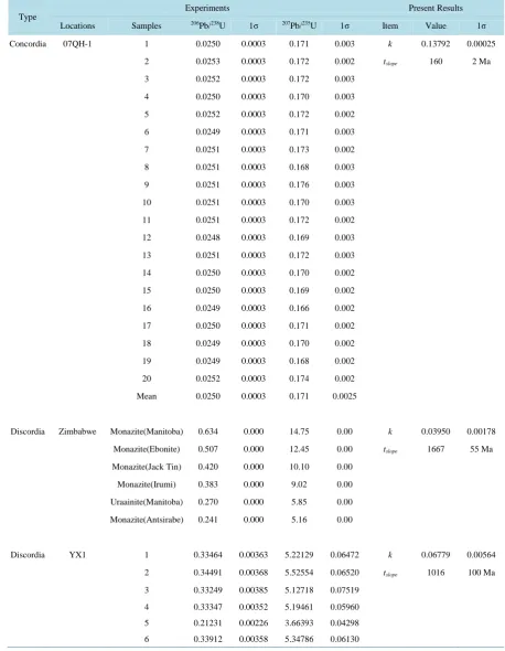
To demonstrate the validity of our work, four examples are illustrated (Table 2 andFigure 5). Table 2 includes original Pb/U isotope ratios from the published literature along with the slope years (i.e. U-Pb ages) when the samples were formed.

The first example comes from Qinghu granite in the Nanling Range, South China [44]. The Pb/U ratios in this granite are the concordant type (Figure 5(a)) [44]. The slope and slope year were calculated using Equations (24) and (10), respectively, and found to be kConcordia = 0.13792 ± 0.00025 and tslope= 160 ± 2 Ma (Table 2), which

(a) (b)

[image:9.595.90.532.80.470.2]

(c) (d)

Figure 5.Present slope years (with 1σ error) for (a) Qinghu granite, (b) a Zimbabwe uranium deposit, (c) Yingxian amphi-bolites and (d) Hebi amphiamphi-bolites. All data points except Zimbabwe are plotted with 1σ error bars. The norms of the residu-als (R2) for the least squares fits are illustrated, and the slopes (with 1σ errors) are given. In (a), the red diamond indicates the mean value for all the measured data and the tangent line at this point coincides with the Concordia line.

The k and tslope values for the three discordant examples described in the introduction were also calculated

using Equations (26) and (10), respectively. For the Zimbabwe uranium deposit (Figure 5(b)), the slope was

kDiscordia= 0.03950 ± 0.00178 and slope year was tslope= 1668 ± 55 Ma. For amphibolites in the Yingxian

lam-proite (YX1,Figure 5(c)), the slope was kDiscordia= 0.06779 ± 0.00564 and slope year was tslope= 1016 ± 100 Ma.

For Hebi amphibolites (HBxa,Figure 5(d)), the slope was kDiscordia= 0.010734 ± 0.00196 and slope year was

tslope= 3237 ± 220 Ma.

4. Conclusion

[image:10.595.80.539.134.725.2]

Table 2. Values for 206Pb/238U, 207Pb/235U, the slope (k) and the slope year (tslope) of zircons in different geological bodies.

The Pb/U isotope ratios in the Qinghu granite (07QH-1), a Zimbabwe uranium deposit, Yingxian amphibolites (YX1) and Hebi amphibolites (HBxa) are taken from Li et al. (2009), Ahrens, (1955), Zheng et al. (2012) and Zheng et al. (2012), re-spectively.

Type

Experiments Present Results

Locations Samples 206_Pb/238_{U 1σ} 207_Pb/235_{U 1σ Item Value 1σ}

Concordia 07QH-1 1 0.0250 0.0003 0.171 0.003 k 0.13792 0.00025

2 0.0253 0.0003 0.172 0.002 tslope 160 2 Ma

3 0.0252 0.0003 0.172 0.003

4 0.0250 0.0003 0.170 0.003

5 0.0252 0.0003 0.172 0.002

6 0.0249 0.0003 0.171 0.003

7 0.0251 0.0003 0.173 0.002

8 0.0251 0.0003 0.168 0.003

9 0.0251 0.0003 0.176 0.003

10 0.0251 0.0003 0.170 0.003

11 0.0251 0.0003 0.172 0.002

12 0.0248 0.0003 0.169 0.003

13 0.0251 0.0003 0.172 0.003

14 0.0250 0.0003 0.170 0.002

15 0.0250 0.0003 0.169 0.002

16 0.0249 0.0003 0.166 0.002

17 0.0250 0.0003 0.171 0.002

18 0.0249 0.0003 0.170 0.002

19 0.0249 0.0003 0.168 0.002

20 0.0252 0.0003 0.174 0.002

Mean 0.0250 0.0003 0.171 0.0025

Discordia Zimbabwe Monazite(Manitoba) 0.634 0.000 14.75 0.00 k 0.03950 0.00178

Monazite(Ebonite) 0.507 0.000 12.45 0.00 tslope 1667 55 Ma

Monazite(Jack Tin) 0.420 0.000 10.10 0.00

Monazite(Irumi) 0.383 0.000 9.02 0.00

Uraainite(Manitoba) 0.270 0.000 5.85 0.00

Monazite(Antsirabe) 0.241 0.000 5.16 0.00

Discordia YX1 1 0.33464 0.00363 5.22129 0.06472 k 0.06779 0.00564

2 0.34491 0.00368 5.52554 0.06520 tslope 1016 100 Ma

3 0.33249 0.00385 5.12718 0.07519

4 0.33347 0.00352 5.19461 0.05960

5 0.21231 0.00226 3.66393 0.04298

Continued

7 0.33246 0.00353 5.22593 0.06103

8 0.24655 0.00268 3.94621 0.04940

9 0.30931 0.00328 5.33072 0.06161

10 0.26968 0.00309 4.22308 0.05705

11 0.34094 0.00374 5.29417 0.06276

Discordia Hbxa 1 0.31857 0.00389 6.52978 0.08636 k 0.010734 0.001956

2c 0.37868 0.00542 11.83149 0.19556 tslope 3237 220 Ma

2r 0.35917 0.00452 9.43864 0.13599

3c 0.32201 0.00375 6.60397 0.08699

3r 0.32726 0.00388 6.39918 0.08482

4 0.35923 0.00457 10.94269 0.15946

5 0.33858 0.00402 8.05032 0.10509

6 0.32256 0.00368 6.04709 0.07394

7 0.32507 0.00396 6.51079 0.08888

8 0.29783 0.00355 6.74590 0.09045

9 0.32970 0.00477 7.19338 0.12913

10 0.34275 0.00486 8.54210 0.14216

11 0.31630 0.00412 7.75610 0.12353

12 0.30213 0.00442 7.02483 0.12968

13 0.31948 0.00461 6.22754 0.13341

Acknowledgements

This work was supported by the National Natural Science Foundation of China (Grant Nos. 41303047, 90914010 and 41020134003).

References

[1] Rutherford, E. and Soddy, F. (1903) The Radioactivity of Uranium. Philosophical Magazine, 5, 25-30, 441-445. [2] Audi, G., Bersillon, O., Blachot, J. and Wapstra, A.H. (2003) The Nubase Evaluation of Nuclear and Decay Properties.

Nuclear Physics A, 729, 3-128. http://dx.doi.org/10.1016/j.nuclphysa.2003.11.001

[3] Jaffey, A.H., Flynn, K.F., Glendenin, L.E., Bentley, W.C. and Essling, A.M. (1971) Precision Measurement of Half- Lives and Specific Activities of 235U and 238U. Physical Review C, 4, 1889-1906.

http://dx.doi.org/10.1103/PhysRevC.4.1889

[4] Pomme, S., Garcia-Torano, E., Sibbens, G., Richter, S., Wellum, R., Stolarz, A., et al. (2008) U-234/U-235 Activity Ratios as a Probe for the U-238/U-235 Half-Life Ratio. Journal of Radioanalytical and Nuclear Chemistry, 277, 207- 210. http://dx.doi.org/10.1007/s10967-008-0731-6

[5] Baker, T., Perkins, C., Blake, K.L. and Williams, P.J. (2001) Radiogenic and Stable Isotope Constraints on the Genesis of the Eloise Cu-Au Deposits, Cloncurry District, Northwest Queensland. Economic Geology, 96, 723-742.

http://dx.doi.org/10.2113/96.4.723

[6] Muller, R. (1996) Radiogenic Isotope Geology. Physics Today, 49, 60. http://dx.doi.org/10.1063/1.2807660

[7] Panneerselvam, K., Macfarlane, A.W. and Salters, V.J.M. (2012) Reconnaissance Lead Isotope Characteristics of the Blackbird Deposit: Implications for the Age and Origin of Cobalt-Copper Mineralization in the Idaho Cobalt Belt, United States. Economic Geology, 107, 1177-1188. http://dx.doi.org/10.2113/econgeo.107.6.1177

Zn-Pb-Cu, Volcanic-Hosted Massive Sulphide Deposit, Tasmania, Using Fluid Inclusions, and Stable and Radiogenic Isotopes. Ore Geology Reviews, 25, 89-124. http://dx.doi.org/10.1016/j.oregeorev.2003.11.001

[9] Ahrens, L.H. (1955) Implications of the Rhodesia Age Pattern. Geochimica et Cosmochimica Acta, 8, 1-15.

http://dx.doi.org/10.1016/0016-7037(55)90013-2

[10] Mezger, K. and Krogstad, E.J. (1997) Interpretation of Discordant U-Pb Zircon Ages: An Evaluation. Journal of Metamorphic Geology, 15, 127-140. http://dx.doi.org/10.1111/j.1525-1314.1997.00008.x

[11] Tilton, G.R. (1960) Volume Diffusion as a Mechanism for Discordant Lead Ages. Journal of Geophysical Research,

65, 2933-2945. http://dx.doi.org/10.1029/JZ065i009p02933

[12] Wetherill, G.W. (1956) An Interpretation of the Rhodesia and Witwatersrand Age Patterns. Geochimica et Cosmochi- mica Acta, 9, 290-292. http://dx.doi.org/10.1016/0016-7037(56)90029-1

[13] Goldich, S.S. and Fischer, L.B. (1986) Air-Abrasion Experiments in U-Pb Dating of Zircon. Chemical Geology, 58, 195-215. http://dx.doi.org/10.1016/0168-9622(86)90010-2

[14] Goldrich, S.S. and Mudrey, M.G. (1972) Dilatancy Model for Discordant U-Pb Zircon Ages. In: Tugarinov, A.I., Ed.,

Contributions to Recent Geochemistry and Analytical Chemistry, Nauka Publishing Office, Moscow, 415-418. [15] Holmes, A. (1954) The Oldest Dated Minerals of the Rhodesian Shield. Nature, 173, 612-614.

http://dx.doi.org/10.1038/173612a0

[16] Silver, L.T. and Deutsch, S. (1961) Uranium-Lead Method on Zircons. Annals of the New York Academy of Sciences,

91, 279-283.

[17] Wasserburg, G.J. (1963) Diffusion Processes in Lead-Uranium Systems. Journal of Geophysical Research, 68, 4823- 4846.

[18] Chew, D.M., Sylvester, P.J. and Tubrett, M.N. (2011) U-Pb and Th-Pb Dating of Apatite by LA-ICPMS. Chemical Ge- ology, 280, 200-216. http://dx.doi.org/10.1016/j.chemgeo.2010.11.010

[19] Thomson, S.N., Gehrels, G.E., Ruiz, J. and Buchwaldt, R. (2012) Routine Low-Damage Apatite U-Pb Dating Using Laser Ablation-Multicollector-ICPMS. Geochemistry, Geophysics, Geosystems, 13, 1.

http://dx.doi.org/10.1029/2011GC003928

[20] Allibon, J., Ovtcharova, M., Bussy, F., Cosca, M., Schaltegger, U., Bussien, D., et al. (2011) Lifetime of an Ocean Is-land Volcano Feeder Zone: Constraints from U-Pb Dating on Coexisting Zircon and Baddeleyite, and 40AR/39AR Age Determinations, Fuerteventura, Canary Islandssp. Canadian Journal of Earth Sciences, 48, 567-592.

http://dx.doi.org/10.1139/E10-032

[21] Bayanova, T.B. and Yakovenchuk, V.N. (1994) U-Pb Dating of Baddeleyite and Zircon from Imandrites on the Kola Peninsula. Doklady Earth science sections, 323, 147-150.

[22] de Assis Janasi, V., de Freitas, V.A. and Heaman, L.H. (2011) The Onset of Flood Basalt Volcanism, Northern Parana Basin, Brazil: A Precise U-Pb Baddeleyite/Zircon Age for a Chapeco-Type Dacite. Earth and Planetary Science Let-ters, 302, 147-153. http://dx.doi.org/10.1016/j.epsl.2010.12.005

[23] Li, Q.-L., Li, X.-H., Liu, Y., Tang, G.-Q., Yang, J.-H. and Zhu, W.-G. (2010) Precise U-Pb and Pb-Pb Dating of Phan-erozoic Baddeleyite by SIMS with Oxygen Flooding Technique. Journal of Analytical Atomic Spectrometry, 25, 1107- 1113. http://dx.doi.org/10.1039/b923444f

[24] Soderlund, U. (2006) U-Pb Baddeleyite Ages of Meso- and Neoproterozoic Dykes and Sills in Central Fennoscandia: A Review. 5th International Dyke Conference: Dyke Swarms—Time Markers of Crustal Evolution, IDC-5. Rovaniemi, 31July 2005-3 August 2005, 75-84.

[25] Wahlgren, C.H., Heaman, L.M., Kamo, S. and Ingvald, E. (1996) U-Pb Baddeleyite Dating of Dolerite Dykes in the Eastern Part of the Sveconorwegian Orogen, South-Central Sweden. Precambrian Research, 79, 227-237.

http://dx.doi.org/10.1016/0301-9268(95)00094-1

[26] Aleinikoff, J.N., Lack, J.F.S., Lund, K., Evans, K.V., Fanning, C.M., Mazdab, F.K., et al. (2012) Constraints on the Timing of Co-Cu Au Mineralization in the Blackbird District, Idaho, Using SHRIMP U-Pb Ages of Monazite and Xenotime Plus Zircon Ages of Related Mesoproterozoic Orthogneisses and Metasedimentary Rocks. Economic Geol-ogy, 107, 1143-1175. http://dx.doi.org/10.2113/econgeo.107.6.1143

[27] Baltybaev, S.K., Levchenkov, O.A., Glebovitskii, V.A., Rizvanova, N.G., Yakubovich, O.V. and Fedoseenko, A.M. (2010) Timing of the Regional Postmigmatitic K-Feldspar Mineralization on the Base of U-Pb Dating of Monazite (Metamorphic Complex of the Northern Ladoga Region). Doklady Earth Sciences, 430, 186-189.

http://dx.doi.org/10.1134/S1028334X1002008X

[28] Bose, S., Dunkley, D.J., Dasgupta, S., Das, K. and Arima, M. (2011) India-Antarctica-Australia-Laurentia Connection in the Paleoproterozoic-Mesoproterozoic Revisited: Evidence from New Zircon U-Pb and Monazite Chemical Age Data from the Eastern Ghats Belt, India. Bulletin of the Geological Society of America, 123, 2031-2049.

[29] Dunning, G.R., Macdonald, A.S. and Barr, S.M. (1995) Zircon and Monazite U-Pb Dating of the Doi Inthanon Core Complex, Northern Thailand: Implications for Extension within the Indosinian Orogen. Tectonophysics, 251, 197.

http://dx.doi.org/10.1016/0040-1951(95)00037-2

[30] Evans, J. and Zalasiewicz, J. (1996) U-Pb, Pb-Pb and Sm-Nd Dating of Authigenic Monazite: Implications for the Dia- genetic Evolution of the Welsh Basin. Earth and Planetary Science Letters, 144, 421.

http://dx.doi.org/10.1016/S0012-821X(96)00177-X

[31] Peterman, E.M., Mattinson, J.M. and Hacker, B.R. (2012) Multi-Step TIMS and CA-TIMS Monazite U-Pb Geochrono- logy. Chemical Geology, 312-313, 58-73. http://dx.doi.org/10.1016/j.chemgeo.2012.04.006

[32] Rasmussen, B., Fletcher, I.R. and McNaughton, N.J. (2001) Dating Low-Grade Metamorphic Events by SHRIMP U-Pb Analysis of Monazite in Shales. Geology, 29, 963-966.

http://dx.doi.org/10.1130/0091-7613(2001)029<0963:DLGMEB>2.0.CO;2

[33] Rasmussen, B., Fletcher, I.R., Muhling, J.R., Mueller, A.G. and Hall, G.C. (2007) Bushveld-Aged Fluid Flow, Peak Metamorphism, and Gold Mobilization in the Witwatersrand Basin, South Africa: Constraints from in Situ SHRIMP U-Pb Dating of Monazite and Xenotime. Geology, 35, 931-934. http://dx.doi.org/10.1130/G23588A.1

[34] Baumgartner, R., Romer, R.L., Moritz, R., Sallet, R. and Chiaradia, M. (2006) Columbite-Tantalite-Bearing Granitic Pegmatites from the Serido Belt, Northeastern Brazil: Genetic Constraints from U-Pb Dating and Pb Isotopes. Cana-dian Mineralogist, 44, 69-86. http://dx.doi.org/10.2113/gscanmin.44.1.69

[35] Camacho, A., Baadsgaard, H., Davis, D.W. and Cerny, P. (2012) Radiogenic Isotope Systematics of the Tanco and Sil- verleaf Granitic Pegmatites, Winnipeg River Pegmatite District, Manitoba. Canadian Mineralogist, 50, 1775-1792.

http://dx.doi.org/10.3749/canmin.50.6.1775

[36] Melcher, F., Graupner, T., Henjes-Kunst, F., Oberthur, T., Sitnikova, M., Gabler, E., et al. (2008) Analytical Finger-print of Columbite-Tantalite (Coltan) Mineralisation in Pegmatites—Focus on Africa. 9th International Congress for Applied Mineralogy, ICAM 2008, 8-10 September2008, Brisbane, 615-624.

[37] Melleton, J., Gloaguen, E., Frei, D., Novak, M. and Breiter, K. (2012) How Are the Emplacement of Rare-Element Pegmatites, Regional Metamorphism and Magmatism Interrelated in the Moldanubian Domain of the Variscan Bohe-mian Massif, Czech Republic? Canadian Mineralogist, 50, 1751-1773. http://dx.doi.org/10.3749/canmin.50.6.1751

[38] Schmitt, A.K. and Zack, T. (2012) High-Sensitivity U-Pb Rutile Dating by Secondary Ion Mass Spectrometry (SIMS) with an O2

+

Primary Beam. Chemical Geology, 332-333, 65-73. http://dx.doi.org/10.1016/j.chemgeo.2012.09.023

[39] Essex, R.M. and Gromet, L.P. (2000) U-Pb Dating of Prograde and Retrograde Titanite Growth during the Scandian O- rogeny. Geology, 28, 419-422. http://dx.doi.org/10.1130/0091-7613(2000)28<419:UDOPAR>2.0.CO;2

[40] Nesterova, N.S., Kirnozova, T.I. and Fugzan, M.M. (2011) New U-Pb Titanite Age Data on the Rocks from the Kare-lian Craton and the Belomorian Mobile Belt, Fennoscandian Shield. Geochemistry International, 49, 1161-1167.

http://dx.doi.org/10.1134/S0016702911120081

[41] Spencer, K.J., Hacker, B.R., Kylander-Clark, A.R.C., Andersen, T.B., Cottle, J.M., Stearns, M.A., et al. (2013) Cam-paign-Style Titanite U-Pb Dating by Laser-Ablation ICP: Implications for Crustal Flow, Phase Transformations and Titanite Closure. Chemical Geology, 341, 84-101. http://dx.doi.org/10.1016/j.chemgeo.2012.11.012

[42] Richards, J.P., Cumming, G.L., Krstic, D., Wagner, P.A. and Spooner, E.T.C. (1988) Pb Isotope Constraints on the Age of Sulfide Ore Deposition and U-Pb Age of Late Uraninite Veining at the Musoshi Stratiform Copper Deposit, Central African Copper Belt, Zaire. Economic Geology, 83, 724-741. http://dx.doi.org/10.2113/gsecongeo.83.4.724

[43] Votyakov, S.L., Ivanov, K.S., Khiller, V.V., Bochkarev, V.S. and Erokhin, Y.V. (2011) Chemical Microprobe Th-U- Pb Age Dating of Monazite and Uraninite Grains from Granites of the Yamal Crystalline Basement. Doklady Earth Sciences, 439, 994-997. http://dx.doi.org/10.1134/S1028334X1107018X

[44] Li, X.-H., Li, W.-X., Wang, S.-C., Li, Q.-L., Liu, Y. and Tang, G.-J. (2009) Role of Mantle-Derived Magma in Genesis of Early Yanshanian Granites in the Nanling Range, South China: In Situ Zircon Hf-O Isotopic Constraints. Scientia Sinica Terrae, 39, 872-887. http://dx.doi.org/10.1007/s11430-009-0117-9

[45] Zheng, J.P., Griffin, W.L., Ma, Q., O’Reilly, S.Y., Xiong, Q., Tang, H.Y., et al. (2012) Accretion and Reworking be-neath the North China Craton. Lithos, 149, 61-78. http://dx.doi.org/10.1016/j.lithos.2012.04.025

[46] Compston, W., Williams, I.S. and Clement, S.W. (1982) U-Pb Ages within Single Zircons Using a Sensitive High Mass-Resolution Ion Microprobe. The 30th Annual Conference on Mass Spectrometry and Allied Topics, Abstracts, Honolulu, 15 February 1984, B525-B534.

[47] Compston, W., Williams, I.S. and Meyer, C. (1984) U-Pb Geochronology of Zircons from Lunar Breccia 73217 Using a Sensitive High Mass-Resolution Ion Microprobe. Journal of Geophysical Research, 89, 525-534.

http://dx.doi.org/10.1029/JB089iS02p0B525

http://dx.doi.org/10.1016/0016-7037(93)90553-9

[49] Srinivasan, G., Whitehouse, M.J., Weber, I. and Yamaguchi, A. (2004) U-Pb and Hf-W Chronometry of Zircons from Eucrite A881467. The 35th Lunar and Planetary Science Conference, League City, TX, 19 March 2004, 1709. [50] Fong, C.F.C.M., Kee, D.D. and Kaloni, P.N. (2002) Advanced Mathematics for Engineering and Science. World

Sci-entific Publishing Co. Pte. Ltd, Singapore.

[51] Wang, J., Qian, Z., Qian, W., Zhuang, Y., He, Y. and Pan, C. (1999) Analysis of Regression and Variance, in Probabil-ity Statistics (Engineering Mathematics). Tongji UniversProbabil-ity, Shanghai, 240-247. (In Chinese)

[52] Bühlmann, P. and Mächler, M. (2008) Computational Statistics, 4-10.

Appendix A: Standard Error (1σ) for the Slope

Using the Least Squares Method

The least squares method is described in textbooks on probability statistics [51] [52]. For a measured set of val-ues (x1, y1,) … (xn,yn), there is a line:

Y=kx+b (A.1)

that best fits the data. The quality of this line is determined by

( )

(

)

2

1 ,

n

i i

i

Q k b y kx b

=

 

=

∑

_ − + _ . (A.2)

When Q k b

(

,

)

is at its minimum value, the estimation (Equation (A.1)) is the “best” fitting of the measured data. This approach is referred to as the method of linear-least-squares.

To find the minimum value for Q k b

(

,

)

, the following equation must be solved:

( )

(

) ( )

( )

(

) (

)

1

1

, 2 0

, 2 0

n

i i

i

n

i i i

i

Q k b y kx b

b

Q k b y kx b x

k = = ∂  _{=  − +  − =} _∂     ∂  _{=  − +  − =}   ∂ 

∑

∑

(A.3)

giving

(

)(

)

(

)

1 2 1 n i i i n i i

x x y y

k

x x

b y kx

= =  _{− −}   =   ₋   = − 

∑

∑

, (A.4)

where 1

n

i i

x x n

=

=

∑

and

1

n

i i

y y n

=

=

∑

. Then Equation (A.1) becomes

(

)

(

)

(

)

1 2 1 n i i i n i i

x x Y Y

k

x x

b Y kx

= =  _{− −}   =   ₋   = − 

∑

∑

. (A.5)

The variance of a new predicted Y_i then follows:

( )

(

)

(

)

(

)(

)

(

)

2 2 2 1 2 1 2 1 1 1 i n n i i

i i n

i i

i Y i n

i

i i

x x y y

y Y

D Y y y

n n

x x

σ = =

= =  _{ }  − −   − _{ }     = = = _ − − _ −      

∑

∑

∑

∑

, (A.6)

where σ is the standard error of Yi or

( )

(

)

2 2 1 2 i n i i i i Y y Y D Y n σ = − = = −

∑

, (A.7)

( )

(

)

(

)

(

)

{

}

(

)

( )

(

)

(

)

(

)

(

)(

)

(

)

2 1 1

2

2 2

2

1 ₁ 1

2 2

1 1

2 2

2

1

1 1

. 2

n n

i i i i

i

i i

k n _n n

i _i i

i _i i

n n

i i

i

i i

n _n

i

i i

i

x x Y D x x Y

D Y

D k D

x x _{x x} x x

x x y y

y y

n

x x _{x x}

σ = =

= ₌ =

= =

= ₌

 ₋  ₋

 

 

= = = =

 ₋  _{  −}

−

  _{ }

  _{ }

 _{ } 

− −

 − _{ } 

 

 

= _ − _

− _{−  }

 _{ − } 

 _{ } 

 

∑

∑

∑

_∑

∑

∑

∑

∑

_∑

(A.8)