Improved Image De noising Algorithm using Dual Tree
Complex Wavelet Transform
B.Chinnarao
Assoc. Prof., Dept of ECE Gokul Institute of Tech. & SciencesBobbili, Vizianagaram, AP, India
M.Madhavilatha,
PhDProf. & Head, Dept of ECE JNTUH College of Engineering
Hyderabad, AP, India
ABSTRACT
Image denoising methods are used to remove the noise components without affecting the important image features and content. Wavelet transforms represents image energy in compact way and this representation helps to find threshold between noisy feature and important image features. In this work we proposed a contextual information based thresholding method in Dual tree complex wavelet transform. We compared our method with other two denoising methods. For comparison purpose we used two standard image processing images using different Gaussian noise variance.
Keywords
NeighShrinkSure; dual tree complex wavelet; thresholding.
1.
INTRODUCTION
An image is often corrupted by noise in its acquisition and transmission. Image denoising is used to remove the noise while retaining as much as possible the important information present in the images. In literature, image denoising methods are based on image characteristic, noise statistical property and frequency spectrum distribution in the images. These methods are divided into two categories, (i) Spatial domain based methods and (ii) Transformation domain based methods. The spatial domain based methods performs data operation on the original image, and processes the image grey value. Neighborhood average method, wiener filter [8] and center value filter are some popular spatial domain methods. In the transformation domain methods, first image transform into another domain and performed some operations on the coefficients (which calculate after transformation processed) [1], [2]. After this we take the inverse transform to go back to image domain. Fouriertransform and wavelet transforms are most popular transformation methods used for image denoising. Wavelet based thresholding methods for image denoising is very popular because wavelet provides an appropriate basis for separating noisy signal from the image signal. Wavelet based methods have advantage over Fourier based methods because wavelet transform gives simultaneous localizationin time and frequency domain and wavelet basis represents energy in compact form. Wavelet coefficients are divided into two group’s first, large coefficients which represent important image features second, small coefficients which mainly represents noise features. Image denoising using thresholding methods means find appropriate value (threshold) which separates noise values to actual image values without affecting the significant features of the image. There are two main types of wavelet transform; continuous
for image denoising because of discrete nature of images presents now days. In this work, we proposed novel thresholding techniques applying on Dual tree complex wavelet coefficients. Dual tree complex wavelet has some advantage over discrete wavelet transform which we discuss later.
This paper is organized as follows: first discussed discrete wavelet transform and its problems, second dual tree complex transform, third thresholding algorithm for image denoising and fourth experiments and results on standard lena and barbara images.
2.
DISCRETE WAVELET TRANSFORM
AND ITS PROBLEMS [3] [4]
Discrete wavelet transform (DWT) used locally oscillating basis functions called wavelets for decomposition of signals. There are two types of functions in wavelets (i) real valued band pass function called mother wavelet(or simply wavelet) ψ(t) and (ii) real valued low pass scaling function φ(t). Any finite energy signal x (t) can be decomposed in terms of wavelets and scaling function as follows.
n) t j Ψ(2 0
j
j/2 2 n d(j,n) n c(n)φ(t n) (t)
x
(1)
Scaling coefficients c (n) and wavelet coefficients d (j, n) are computed as follows
dt n) (t φ x(t)
c(n)
(2)
2j/2 x(t)ψ(2jt n)dt n)
d(j,
(3) J is scale factor, which controlled frequency content, and n controlled the time shift
In 2D wavelet transforms the scaling and wavelet functions are two variable functions φ(x, y) and ψ(x, y). In DWT, an image is filtered into four sub bands at each resolution and the sub band which has lowest frequency sub band is further subdivided through an iterative process to provide the multi resolution representation
M 1
0
x (x,y)
1 N
0
y φj0,m,n y) f(x, MN
1 n) m, , 0 (j φ
W (4)
H,V,D
i, 1
M
0
x (x,y)
1 N
0
y φ
i n m, j, y) f(x, MN
1 n) m, (j, i ψ
W
(5) The image is decomposed into four sub band: Wφ (j, m, n) denotes the low frequency approximation and WψH
, WψD, WψV
denotes the high frequency sub bands in horizontal (H), vertical (V) and diagonal (V) orientation (Fig 1)
There are four problems in discrete wavelet transform as follows:
1. Wavelets are band pass functions, due to this wavelet coefficients shows oscillating nature (positive and negative) around singularities 2. Small shift in signal causes large change in
wavelet coefficients.
3. Processing in wavelet domain such as thresholding and filtering cause the aliasing artifacts.
4. Wavelet lacks the directionality in higher dimensions.
These four problems in DWT can resolve by using complex wavelet basis function instead of real function basis function which used in DWT transform [6]. Due to using complex scaling and wavelet function (Ψc (t)) this transform called complex wavelet transform.
Ψc(t)Ψr(t)jΨi(t) (6) Ψr (t) are real and even and j Ψi (t) are imaginary and odd function. Ψr (t) and Ψi (t) are formed a Hilbert transform pair (90° out of phase each others) and wavelet function (Ψc (t)) is called the analytics signal.
The two real wavelet transforms use two different sets of filters. [7] The two sets of filters are jointly designed so that the overall transform is approximately analytic. Let h0 (n), h1 (n) denote the low-pass/high-pass filter pair for the upper FB, and let g0 (n), g1 (n) denote the low-pass/high-pass filter pair for the lower FB. Denote the two real wavelets associated with each of the two real wavelet transforms as ψh(t) & ψg(t). Filters are designed so that the complex wavelet
ψ(t ) = ψh(t ) + j ψg(t)
Equivalently, they are designed so that ψg(t) is approximately the Hilbert transform of ψh(t) [denoted ψg(t) ≈ H{ψh(t)}] If the two real DWTs are represented by the square matrices FK and Fg, then the dual-tree CWT can be represented by the rectangular matrix
g F
h F
F (7)
If the vector x represents a real signal, then wh = Fh x represents the real part and wg = Fgx represents the imaginary part of the dual-tree CWT. The complex coefficients are given by wh + j wg.
Fig 2: Dual tree CWT as filter bank approach
3.
IMAGE DENOISING ALGORITHM
This section describes image denoising algorithm. Image denoising means usually compute the soft threshold such a way that information presents in image is preserved. Typical pipeline for image denoising using wavelets as follows (Fig 3):
1. first decompose noise corrupted image using multi resolution wavelet transform
2. Calculate soft threshold in wavelet domain and apply to noisy coefficients.
3. Apply inverse wavelet transform to reconstruct image in spatial domain.
[image:2.595.55.280.226.316.2]In this work we proposed a new soft thresholding algorithm using Dual tree complex wavelet transform.
When wavelet transform is computed for varying sub bands, the first few coefficients posses the key information which can be used for denoising. The noise is estimated from the coefficient by posing it as an estimation problem. Assuming the coefficients are the product of a random process, the underlying noiseless distribution is estimated using robust estimator. Two problems have to address when such an algorithm is designed. What is the neighborhood of the handful of coefficients to be considered during the estimation process and how many coefficients would suffice the task. The algorithm (Fig 4) mentioned below addresses these challenges by assuming an additive Gaussian Noise distribution on the data and adaptively chooses the number of coefficients and the neighbor-hood.
For each window size L x L compute the threshold as follows; 1. Let θ is the noiseless coefficients and σ is the
noisy coefficients.
2. We want to minimize E{|| θ – σ||22} function where E{} is expected loss
3. We can write expected loss as follows a. E{|| θ – σ||2
2} = Ns + E{wavelet energy within window + gradient(wavelet energy within window
b. Wavelet energy within widow =
ij
θ
2
ij
W
[image:3.595.59.282.277.717.2]c. Noise parameter estimated from the noise content through median absolute deviation (MAD) estimation. We minimize this expectation function E {} through M-robust estimator. Thus the amount of denoising is controlled by local primitives of the image
Fig 4: Algorithm flow chart.
In this work we proposed a denoising algorithm on dual tree complex wavelet domain. For computing threshold we used
Noise parameter estimation using MAD estimator a following equation
, yi subban
d
0.6745 ) i y ( median 2 n
σ
(8)
4. RESULTS
The performance of thresholding algorithm proposed by us is tested on two standard images (Lena and Barbara) used in image processing. Gaussian noise with zero mean and different variances is used for performance evaluation. Image size is 512 x 512 and for performance evaluation PSNR (peak signal to noise value) and SSIM values are used.
PSNR values is calculated as follows
dB MSE 2 255 10 10log
P SNR
(9)
Where, MSE is the mean square error which is the difference between original image and reconstructed image. Second measure SSIM is used because natural image signals are highly structured: Their pixels exhibit strong dependencies, especially when they are spatially proximate, and these dependencies carry important information about the structure of the objects in the visual scene. The Minkowski error metric is based on point wise signal differences, which are independent of the underlying signal structure. Although most quality measures based on error sensitivity decompose image signals using linear transformations, these do not remove the strong dependencies; the motivation of our new measure is to find a more direct way to compare the structures of the reference and the distorted signals.
) 2 C 2 Y σ 2 X )(σ 1 C 2 Y μ 2 X (μ ) 2 C XY )(2σ 1 C Y μ X (2μ Y X, SSIM (10)
Where x represents original image and y represents distorted image.
considerably superior to Neigh Shrink and also outperforms SURE-LET, which is an up-to-date denoising algorithm based on the SURE. It is well known that increasing the redundancy of wavelet transforms can significantly improve the denoising performances. As the results shown in table 1, 2, 3, 4 that our method performs better in comparison to other two methods discussed above. We have used two performance measures PSNR and SSIM to compare the performance of the three image denoising techniques. The experimental results in Peak Signal to Noise Ratio (PSNR) and Structural Similarity Index [11] (SSIM) are shown in Table 1-IV and Figure 5(a) to 5(e).
Table 1. Comparison for Lena Image (PSNR in dB)
Noise, σ Wiener
filter
NeighShrink Sure
Proposed method
10 33.62 34.72 35.34
15 31.17 32.87 33.62
20 29.03 31.53 32.37
25 27.24 30.53 31.38
30 25.74 29.70 30.53
35 24.45 29.01 29.86
40 23.33 28.41 29.26
45 22.33 27.84 28.69
[image:4.595.46.287.228.467.2]50 21.44 27.43 28.14
Table 2. Comparison for Barbara Image (PSNR in dB)
Noise, σ Wiener
filter
Neigh Shrink Sure
Proposed method
10 29.91 33.02 33.73
15 28.33 30.69 31.49
20 26.85 29.09 29.98
25 25.52 27.93 28.77
30 24.33 29.01 27.88
35 23.27 26.25 27.06
40 22.32 25.62 26.36
45 21.47 21.86 25.87
50 20.70 24.63 25.34
Table 3. Comparison for Lena Image (SSIM)
Table 3. Comparison for Barbara image (SSIM)
Noise, σ Wiener
filter NeighShrinkSure
Proposed method
10 0.94 0.96 0.97
15 0.90 0.94 0.95
20 0.85 0.92 0.93
25 0.80 0.89 0.90
30 0.75 0.87 0.88
35 0.70 0.85 0.87
40 0.65 0.82 0.85
45 0.61 0.80 0.83
50 0.57 0.78 0.81
As noise variance increases the performance of our method improves because we compute the threshold in complex dual tree wavelet transform domain which has advantages over DWT domain and using spatial context information. Spatial context information helps to predict the actual values (noiseless value while using all neighborhood information presents in working window. Experimental results indicate that the proposed adaptive denoising method (DT-CWT) yields the better performance than some of the already published best denoising algorithms. This new technique maintains the simplicity, efficiency and intuition of the classical soft thresholding approach.
Noise, σ Wiener
filter NeighShrinkSure
Proposed method
10 0.94 0.96 0.96
15 0.89 0.94 0.95
20 0.83 0.92 0.93
25 0.76 0.90 0.91
30 0.70 0.88 0.90
35 0.65 0.86 0.88
40 0.60 0.84 0.87
45 0.55 0.83 0.85
[image:4.595.48.288.497.740.2]Fig 5 (a): Original Lena image
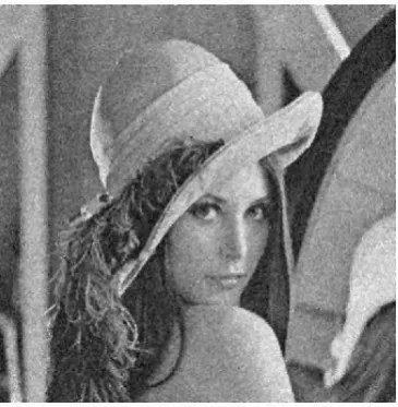
Fig 5 (b): Lena image with noise variance 30
Fig 5 (c): Proposed algorithm output image
Fig 5 (d): Denoised using NeighShrinkSure method
[image:5.595.358.534.84.238.2]Fig 5 (e): Denoised using Wiener filter method [image:5.595.362.545.292.479.2]
Fig 7: SSIM Performance of all three methods
5. CONCLUSION
In this work we proposed a new soft thresholding method for image denoising using complex dual tree wavelet transform domain. Our method has advantage of complex wavelet function which is motivated by complex basis of Fourier transform. While using complex basis function we have less artifacts and ringing artifacts for reconstruction of image. Images normally have strong contextual information which was utilized while calculating threshold. Our method is highly suitable at high noise levels compared to low noise levels.
6. REFERENCES
[1] Donoho.D.L,Johnstone.I.M, “Ideal spatial adaptation via
wavelet shrinkage”, Biometrika,81,pp.425-455,1994.
[2] Aglika Gyaourova Undecimated wavelet transforms for image denoising, November 19, 2002.
[3] C Sidney Burrus, Ramesh A Gopinath, and Haitao Guo, “Introduction to wavelet and wavelet transforms”, Prentice Hall1997.
[4] S. Mallat, A Wavelet Tour of Signal Processing, Academic, New York, second edition, 1999.
[5] R. C. Gonzalez and R. Elwood‟s, Digital Image
Processing. Reading, MA: Addison-Wesley, 1993.
[6] L. Sendur and I.W. Selesnick, "Bivariate shrinkage with local variance estimation," IEEE Signal Proc. Letters, vol. 9, pp. 438- 441, Dec. 2002.
[7] N. G. Kingsbury,” The dual-tree complex wavelet
transform: a new technique for shift invariance and directional filters”, In the Proceedings of the 8th
IEEE Digital Signal Processing Workshop, Bryce Canyon Aug 1998.
[8] J. Neumann and G. Steidl, ”Dual–tree complex wavelet
transform in the frequency domain and an application to signal classification”, International Journal of Wavelets, Multiresolution and Information Processing IJWMIP, 2004.
[9] Javier Portilla, Vasily Strela, Martin J. Wainwright, Eero P. Simoncelli, Adaptive Wiener Denoising using a Gaussian Scale Mixture Model in the wavelet Domain, Proceedings of the 8th International Conference of Image Processing Thessaloniki, Greece. October 2001.
[10] Zhou Dengwen, Cheng Wengang, "Image denoising with
an optimal threshold and neighbouring
window," Pattern Recognition Letters, vol.29, no.11, pp.1694–1697, 2008
[11] Zhou Wang, Alan C. Bovik, Hamid R. Sheikh, Eero P. Simoncelli,’’ Image Quality Assessment: From Error Visibility to Structural Similarity
[12] Zhou Dengwen ,An Image Denoising Algorithm with an adaptive window IEEE 2007
7. AUTHOR S PROFILE
B. Chinna Rao is currently pursuing PhD from JNTU. He has been actively guiding students in the area of Signal and Image Processing. He has published 3 international journals and attended 6 International Conferences. Currently, he has been working as Assoc. Professor in Dept. of Electronics & Communication engineering In Gokul Institute of Technology & Sciences Bobbili, Vizianagaram Dist, Andhra Pradesh, India.
Dr. M. Madhavi Latha is specialized in signal and image processing using wavelets and Low Power Mixed Signal Design in VLSI. She has published 35 publications in various journals and conferences at national and International level and presented papers in conferences held at Losvegas, Louisiana, USA and Iunstrruck, Austria
presently