Development of Altman Five Factor Model of Assessing the Creditworthiness of an Enterprise

(1)

http://dx.doi.org/10.4236/me.2015.67075

Development of Altman Five-Factor Model

of Assessing the Creditworthiness of an

Enterprise

Boureima Bamadio, Konstantin Andreyevich Lebedev

Department of Computational Mathematics and Informatics, Kuban State University, Krasnodar, Russia Email: [email protected], [email protected]

Received 14 June 2015; accepted 12 July 2015; published 15 July 2015

This work is licensed under the Creative Commons Attribution International License (CC BY). http://creativecommons.org/licenses/by/4.0/

Abstract

In this paper, we propose a method that uses the apparatus of the theory of fuzzy sets, together with the five-factor model of Altman to assess the creditworthiness of an enterprise. Altman’s mo- del is enhanced in two ways: applies integral approximation of the root mean square for the exact calculation of quantitative credit assessment (probability of bankruptcy), and applies the device of fuzzy sets for ordered sets according to the degree of confidence in the resulting probability. Some real examples of the methodology of applications are shown. The article is theoretical in nature, the findings made in the mathematical model have not been tested on a sufficiently large number of enterprises.

Keywords

Estimation of Credit Status of a Company, Altman Model, Fuzzy Sets, Integral Mean-Square Approximation, Newton Method

1. Introduction

Presently, timely return of loans is an urgent problem for all the creditor institutions (banks). To a large extent, solution to this problem depends on the “quality” of a reliable assessment of the creditworthiness of companies, carried out by experts on the basis of their accounting statements. Despite the presence of Russian and foreign number of techniques and models in practice, there is no universal model. Practical application of Altman’s Model in the Russian condition considered in [1] [2].

(2)

the problem of economy and management of enterprises, but application of fuzziness is underutilized when ana-lyzing and evaluating the creditworthiness of businesses [4] [5]. This paper proposes application of theory of fuzzy sets and standard integral approximation for the quantitative assessment of creditworthiness (probability of bankruptcy) of the company. Thus, the purpose of this article is the development (improvement) based on the Altman’s model of the theory of fuzzy sets, mathematical optimization, enabling an effective method to improve the credit assessment (bankruptcy), and offers a way to streamline the fuzzy sets of the calculated measure of preference.

2. Statement of the Problem

In international practice (the US economy), the greatest distribution model has a five-factor model of Altman in order to assess the possibility of bankruptcy, and has the form [6]:

1 2 3 4 5

1.2 1.4 3.3 0.6 1.0

z= k + k + k + k + k , (1)

where the coefficients k_i, i=1,,5, are defined: k₁—net working capital/total assets, k₂—Retained earn-ings/total assets, k₃—profit before interest/total assets, k₄—the market value of equity/debt capital, k₅—vo- lume of sales/total assets. Russia has adapted the model to adjust Altman weight ratios k_i [1].

Altman’s model establishes the dependence of the probability function p z

( )

value of z. This probability is calculated as follows:

( )

[

]

[

]

[

]

[ ]

0.80,1.0 если 0 1.8 0.35, 0.5 если 1.81 2.77 0.15, 0.2 если 2.8 2.99 0, если 3

z z p z

z z

ε

 ≤ ≤

 _{≤ ≤}



=  _{≤ ≤}



 _{≤ < ∞}



, (2)

when z≥3, the probability of bankruptcy, p=

ε

is quite small (

ε

→0 when z→ ∞) and is considered to be approximately equal to zero. Hereinafter we will take

ε

=0.05 for the problem. Figure 1shows the graph of the function p z

( )

of Altman model (1). We define two functions ₁

( )

min

( )

z

f z p z

∀

= , ₂

( )

max

( )

z

f z p z

∀

= .

After this, we will solve the problem mean integrated squared approximation sets of Altman by a polynomial of sufficiently high n-th degree, as follows [7]:

( )

0

n i

i

L z a z

=

∑

(3)

On the interval z∈

[

0,z4

]

,z4=3.5. We select the degree of the polynomial discussed in [7]. The coefficients

were determined from the minimization problem in n-dimensional space _Rn+1_{polynomial coefficients,}

( )

{

1

}

arg min

n

a R

a ₊ F a

∈

= (4)

where,

( )

(

( )

)

4

2

2 1 0

d

z

т i i

F a L z f z z

=

∑ ∫

− , a=

{

a a a₀, ₁, ₂,,a_n

}

T, with additional natural restrictions [7].

( )

_{( )}

( )

4

0

d d

0, 0, 0.

d d

n n

n _{z z}

z z z

L z L z

L z

z ₌ = = = z ₌ = (5)

3. Newton’s Method for Finding the Extrema of Functionals

In the segment on which approximation is made, the right extreme point is selected z₄ =3.5 [7]

The main objective is to transform the minimization problem F a₀

( )

with the relevant restrictions (5) - (7), the task of finding the minimum without limitation function

( )

0

( ) ( )

,

F a =F a +g a (6)

(3)

f2(z)

f1(z)

L(v,z)

f2(z)

f1(z)

L(v,z)

f2(z) f1(z)

L(v,z) f2(z)

f1(z)

L(v,z)

0.5 1 1.5 2 2.5 3 3.5

z 0 0.5 1 1.5 2 2.5 3 z 3.5

0 0.5 1 1.5 2 2.5 3 _z 3.5

0 0.2 0.4 0.6

0 0.8 1 1.2

0.2 0.4 0.6

0 0.8 1 1.2

0.2 0.4 0.6

0 0.8 1 1.2

0.2 0.4 0.6

0 0.8 1 1.2

(a) Graph of polynomial L3(z) (b) Graph of polynomial L5(z)

(c) Graph of polynomial L6(z) (d) Graph of polynomial L7(z)

Figure 1.The graph of a function of fuzzy variable p(z) Altman model. The graphs of the functions ₁

( )

min

( )

z

f z p z

∀

= ,

( )

2 max_z

f z p z

∀

= integrated by the method of mean-square approximation polynomials L zn

( )

with different degrees of the polynomial n: (a) 3; (b) 5; (c) 6; (d) 7.

( )

(

( )

)

4 4

2 2

2

1 2 3

0

d , d ,

, .

d d

n n

n _{z z}

z z z

L a z L a z

g a k k k L a z

z ₌ z ₌ =

 

 

= _ _ + +

 

   

(7)

Selecting large penalty coefficients k₁ =1000, k₂=1000, k₃=1000.

Instead, the constrained minimization problem of (4) - (5) solves the problem of unconstrained minimization of the objective function (8).

( )

min₁

n

a R

F a ₊

∈

→ (8)

[image:3.595.78.541.78.516.2]

(4)

se-lection method and thereby solve the challenge of computational mathematics relevant for modification of the classical Newton’s method for calculating the localized extremum convex functions with a view to expanding the area of convergence of iteration [9]. To simplify the proofs of theorems the function assumes an increased supply of smoothness. As a result of the proposed modification, the iterative process based on the method of continuation, should lead to the localization of the desired solution in which the sufficient conditions for the convergence of the classical procedure is satisfied [10].

We assume that the function is strongly convex F G: ⊂Rn+1→R on a convex closed set G⊂Rn+1 normed linear space, which ensures the uniqueness of the local minimum a_*∈G [11]. We assume sufficient smoothness of the strongly convex function F a

( )

in problem (8).

а) _{F a}

( )

_∈_C3

( )

_R

б)

( )

1

xx

F a − ≤M

We assume that the mappings

(

)

: n n, : n n, n , : n n n

xx xxx

F R →R F R →L R R B R ×R →R

are defined by the formulas

( )

n

xx

F a h∈R ,

( )

(

n, n

)

xxx

F ξ h∈L R R , h∈Rn,

ξ

=

{

ξ

1,,

ξ

n

}

, n n R

ξ

∈ ,

( )

( )( )

, n

xxx

F ξ h h=B ξ h h ∈R

    ,

( )

, 1, i xx

i j n

f

F a a

a =

∂

 

= _∂ 

  , Fxxx

( )

ξ =

{

W1

( )

ξ1 ,W2

( )

ξ2 ,,Wn

( )

ξn

}

,

( )

2

, 1,

i k k k

k j _{i j} _n

f W a a

ξ

=  _∂    = _{∂ ∂}      ,

( )

3

( )

, 1,

i

k k k

k i j _{i j} _n

f W

a a a

ξ

=  ∂    = _{∂ ∂ ∂}      ,

where f a

( )

=F ax

( )

, F Fx, xx,Fxxx, fx,fxx—first and second derivative,

(

,

)

n n

L R R —normed linear space of

matrices, B—bilinear operator [10]. m is taken as the norm [11]:

( )

max

( )

max

( )

x xi i

i i

F a = F a = f a ,

( )

1 1 max max n n xi i xx i i

j j j j

F f

F a a a

a a = = ∂ ∂ = = ∂ ∂

∑

,

( )

1 max max n xi xxx

k i _j

k j

F

F a a

a a =  _∂    = _ _ ∂ ∂   

∑

.

In which the formulated conditions a) - б) exist in an area U_*, containing a_*, from any point for which

0 *

a=a ∈U ⊂G classical

(

β

=1

)

the Newton’s method for problem (8) converges to the root a_*, however, the diameter of the area is small [8] [11].

Using the notion and notations, we can prove the theorem as a corollary of theorem [8] on the convergence of the modified (9) - (11) of Newton’s method, given by the following formulas

( )

, 0 ,

xx j j x j

F a ∆ = −a F a a ∈G (9)

1

j j j j

a+ =a + ∆

β

a (10)

( )

₁ 2

( )

1

1,2

min 1, 2 .

j nN Fxx aj F ax j

β

− −  _ _    = _ _ _ _       (11)

A theorem on the convergence of Newton’s method. If the conditions а) - b) are met the process (9) - (11)

for the problem (8) from any point in a finite number a₀∈G of steps j= 1 leads to the initial approximation

0

l

(5)

Proof. If we follow the method of proof of the theorem [8], under the formulated assumptions a) - b), then the proof of the theorem reduces to reference to the fact that the task of finding an extremum with the given as-sumptions is equivalent to the problem of finding the roots of nonlinear equations

( )

0

f a =

with given assumptions а) - d) [8]. а)

( )

2

( )

f a ∈C G ,

b) f_xx

( )

a ≤N,

c) det

(

fx

( )

a

)

≠0, г)

( )

1

x

f a − ≤M

where f a

( )

=F a_x

( )

. a) If

( )

3

( )

F a ∈C G , to

( )

2

( )

f a ∈C G

b) From the functions belonging to the class of three times continuously-differentiable functions

( )

3

( )

F a ∈C G

and the well-known Weierstrass theorem for continuous functions on closed bounded sets [13] [14] we have the estimate F_xxx

( )

a ≤N.

c) If F a

( )

is strongly convex on G, then we evaluate det

(

Fxx

( )

a

)

≠0 (and det

(

fx

( )

a

)

≠0) on G[15].

d) Since we are assuming Fxx

( )

a 1 M

−

≤ then, fx

( )

a 1 M

−

≤ .

All the four conditions for the function f a

( )

=F ax

( )

been satisfied, it follows that the modified Newton’s

process (9) - (11) leads to the region U_* containing a_*, from any point for which a=a₀∈U_*⊂G classical

(

β

=1

)

the Newton’s method will converge to a minimum function F a

( )

.

Thus the theorem is proved for sufficient conditions for the convergence of the modified method of (9), (11). Practical application involves the stopping of the algorithm. The search process is stopped when approx-imately the necessary conditions for an extremum are fulfilled.

x

F <ε

A corollary is formulated for strongly convex functions whose detFxx ≠0, in practice, however, this value

can be very low, especially when used in the reduction of problems with constraints to unconstrained optimiza-tion after applying the method of penalty funcoptimiza-tions. If any funcoptimiza-tional that does not belong to the class of strongly convex functions, then the condition detFxx≠0 cannot be guaranteed over the entire region G. Therefore, it is

feasible to resort to regularization algorithm using small parameter

α

>0.

( )

xx j j x j

E F a a F a

α

 + ∆ = −

  ,

1

j j j j

a+ =a + ∆

β

a

where E is a unit matrix [12].

It follows that the solution of linear equation always exists. Moreover it is possible select the parameters (

α

and β ) and to optimize the process of searching for the extremum, or to ensure that the relaxation properties of the iterative process

( )

j1

( )

j

F a + < F a

It should be noted that the formulas are difficult to use in practice, since the constants N and M usually in problems of practical content, are not always known. However such theorems allow you to specify on the avail-ability principle to resolve one of the most significant shortcomings of the Newton’s method, which is to choose a good initial approximation and offer some ways to do this [8] [12] [13].

Coefficients “a” obtained for a third degree polynomial:

{

} {

T

}

0, 1, 2, 3 1.095; 0; 0.267; 0.051

a= a a a a = −

Figure 1(а); polynomial of fifth degree:

{

}

T

{

₃ ₃

}

0, 1, 2, 3, 4, 5 0.925; 0;8.448 10 ; 0.038; 0.011; 4.309 10

(6)

Figure 1(b); polynomial of sixth degree:

{

}

T

{

3 3 4 4

}

0, 1, 2, 3, 4, 5, 6 0.937; 0; 2.167 10 ; 0.052;1.798 10 ;8.006 10 ;3.132 10

a= a a a a a a a = × − − × − × − × −

Figure 1(c); polynomial of seventh degree:

{

}

{

}

T 0 1 2 3 4 5 6 7

3 3 4 4 4

, , , , , , ,

1; 0.933; 0; 2.0089 10 ; 0.049;1.62 10 ; 6.231 10 ; 2.396 10 ; 2.35 10 ,

a a a a a a a a a

− − − − −

=

= × − × × × ×

Figure 1(d).

FromFigure 1 we see that, the polynomials for n= 6 and n = 7 intersect all four areas. In the case of small or large n, there are some differences: n = 3 in the form of lack of smoothness, the curve is more similar to direct or monitor features functions Altman; n = 5, there are high and some different z has the same value p; n = 9 is too narrow zone, z change outside, of which the function values Altman’s equal to 0 or 1.

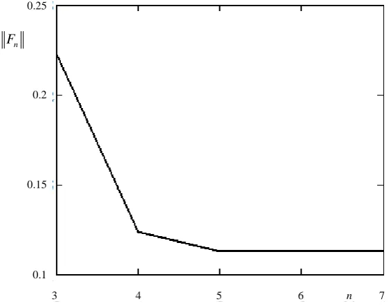
It is noticeable that inFigure 2, the values of the optimization functions are decreasing convergent sequence on the degree of the polynomial, so as soon as the convergence rate becomes small, further increasing the degree of the polynomial becomes meaningless. The degree of the polynomial at which the rate of convergence de-creases is many times clearly visible from the figure of convergence and the value equal 6.

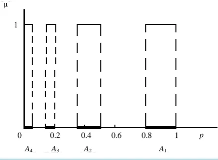
4. The Fuzzy Sets Generated by the Altman Five-Factor Model

In model (1), parameters ki calculated by the parameter z cannot be measured accurately. Therefore, model (1) generates fuzzy sets, which belong to the values of the quantity p, and the values of membership functions of these sets coincide with the probability of bankruptcy. Altman’s model allows a first approximation, the com-pany divided into four classes, with a probability of bankruptcy A_i, i=1,, 4. A₁=

[

0.8,1.0

]

—“High proba-bility of bankruptcy”, A₂=

[

0.35, 0.50

]

—“average probability of bankruptcy”, A₃=

[

0.15, 0.20

]

—“the proba-bility of bankruptcy is not great”, A₄ =

[ ]

0,

ε

—the company “small probability of bankruptcy.” In the example considered p∈

[ ]

0,1 .

For fuzzy sets X_i given by the membership function

( )

:

[ ]

0,1

i

X p U Μ R

µ_ → ∈µ = ∈ , (discussed below in

Section 4). If the value of the probability p, found Altman model (1) using L6(z) falls into one of the sets, the

value of the membership function is equal µ=1. This situation is shown in Figure 3. In this case, the probabil-ity of bankruptcy is attributed to the value obtained p=L z₆

( )

∈A_i. If, p=L z₆

( )

∉A_i, then µ=0.

3 0.1

4 5 6 n 7

0.2 0.25

0.15

n

[image:6.595.171.454.474.695.2]

F

(7)

0 1

0.2 0.4 0.6 0.8 1 p

A4 A3 A2 A1

[image:7.595.200.423.84.247.2]

μ

Figure 3. The values of the membership function at p∈X_i.

The sets A_i are clearly specified by their distribution functions

µ

.

The construction of functions L6(z) is the ability to get the p value in the areas that lie outside of sets Altman,

however, in such cases there is a need to get the value attributed to one of the nearby sets Altman, for which purpose it is proposed to use the theory of fuzzy sets, building the simplest piecewise linear continuous mem-bership function [14]. When the probability value p, was found in Altman model (1) using L6(z) it does not fall

within one of the sets p=L z₆

( )

∉A_i, then the value of the membership function will be located using the fuzzy sets technique presented below (in Section 3). Currently fuzzy sets are actively used in practice in the analysis of risk of bankruptcy of enterprises [15].

4.1. Membership Function

Membership function

µ

_A

( )

u is a function, domain of definition which is the carrier U,

(

u U∈

)

, and the range of values µ_A is the unit interval

[ ]

0;1 [15][16]. The higher the value

µ

_A

( )

u , the higher estimated degree of belonging of an element of the carrier U of the fuzzy set A. In our case we choose as a carrier U =

{

X, 0≤X ≤1

}

, on which a plurality of Ai where u= p—the probability of bankruptcy, corresponding to the value z, found

by the Equation (1). On the media define the membership functions for the values of p₁—

( )

1

X p

µ_ , p₂—

( )

2

X p

µ_ , p₃—

( )

3

X p

µ , p2—µX₄

( )

p ,and the first of them corresponds to a fuzzy subset X1, the second— 2

X , third—X₃, and fourth—X₄, where X₁—“the possibility of bankruptcy is high,” X₂—“average bank-ruptcy”, X₃—“Little possibility of bankruptcy”, X₄—“the possibility of bankruptcy is small”.

Calculating the value z model Altman (1) and calculating p according to the formula L6(z) is not always

poss-ible to carry the calculated value of p in one of the sets Ai, that is one of the cases p∈A1 =

[

0.8,1.0

]

,

[

]

2 0.35, 0.50

p∈A = , p∈A₃=

[

0.15, 0.20

]

, p∈A₄=

[

0, 0.05

]

. For example, if p∈0.7, then p can be attri-buted to set A1 and a set A2.

In this context, we introduce fuzzy sets X_i which defined preference function

( )

:

[ ]

0,1

i

X u U Μ R

µ_ → ∈µ = ∈ , allowing to determine the measure of fuzzy sets X_i, in this case, the measure of fuzziness of the calculated probabilities p=L₆

( )

z ∈X_i.

The membership functions of the subsets, X₁, X₂, X₃, X₄ are of the form:

1

10 5

, 0.5 0.8,

3

1, 0.8 1;

X

p

если p

µ

−

 _{≤ <}

 = 

 _{≤ ≤}



 (6)

2

100 20

, 0.2 0.35,

15

1, 0.35 0.5,

8 10

, 0.5 0.8;

3 X

p

если p

p

если p

µ

−

 _{≤ <}

 

= ≤ <

 −

 ≤ ≤



(8)

3

100 5

, 0.05 0.15,

10

1, 0,15 0, 2,

35 100

, 0.2 0.35,

15 X p если p если p p если p µ −  _{≤ ≤}  

=_ < ≤

 ₋

 < ≤



 (8)

4

1, 0 0.05,

15 100

, 0.05 0.15.

10 X если p p если p

µ

≤ <   = − _{≤ ≤} 

 (9)

Then, we can write many of such sets using the traditional set theory notation (using the integral sign) [15] [16]:

( )

1

0.5 1 0.5 0.8 0.8 1

10 5

1 ; 3

X

p p p

p

X µ p p p p

≤ ≤ ≤ < ≤ ≤

−

 

= = _ _ +

 

∫



∫

 (10)

( )

2

0.2 0.35 0.35 0.5 0.5 0.8

0.2 0.8

100 20 8 10

1 ;

15 3

X

p p p

p

p p

X µ p p p p p

≤ < ≤ ≤ < ≤

≤ ≤ − −     = = _ _ + + _ _    

∫



∫

 (11)

( )

3

0.05 0.35 0.05 0.15 0.15 0.2 0.2 0.35

100 5 35 100

1 ;

10 15

X

p p p p

p p

X µ p p p p p

≤ ≤ ≤ ≤ < ≤ < ≤

− −

   

= = _ _ + + _ _

   

∫



∫

 (12)

( )

4

0 0.15 0 0.05 0.05 0.15

15 100

1 .

10

X

p p p

p

X µ p p p p

≤ ≤ ≤ < ≤ <

−

 

= = + _ _

 

∫



∫

 (13)

See Figure 4 below. If all graphs a) - г) represent on a single coordinate system, the function of the abscissa of the intersection points

( )

i

X p

µ и µX_i+₁

( )

p , will equal to p1 =0.1, p2=0.275, p3=0.65 and they meet

the definition (14) next sets clear X_i₀ (see Section 4.2).

0

0.4 0.6 0.8 p 1

μ(p)

0.5 1

(a)

0

0.4 0.6 0.8 _p 1

μ(p)

0.5 1

0.2 0

0

μ(p)

0.5 1

0

μ(p)

0.5 1

0 0.1 0.2 0.3 _p 0.4 0 0.05 0.1 0.15 p 0.2

(B) (Γ)

(б)

1

X X₂

3

X X4

Figure 4. Plots the membership functions of fuzzy subsets (а) X₁, (б) X₂, (в) X₃, (г)

4

(9)

4.2. Measures of Fuzzy Sets

After calculating z, p(z), choose X_i and calculate the measure of accessories

( )

i

X p

µ_ that will appreciate the sets X_i from the point of view of fuzziness, i.e. we introduce a complete ordering of the sets according to their degree of fuzziness. To determine the degree of fuzziness of sets used its measure of fuzziness d, which is confined to measuring the differences between the Measure of fuzzy sets X and clear set X₀ [15] [16]_{. The} measure of fuzziness of a set X is defined as the distance d X X

(

, ₀

)

from this set to the set X closest to the clearly given set X₀:

(

)

(

)

0

, X, X .

d X X =ρ µ µ A clear subset X0, fuzzy nearest X to the membership

function µ_X_

( )

u

(

µ_i∈M

[ ]

0,1 ⊂R

)

, called the subset X₀∈U, the characteristic feature of which is as fol-lows:

0

1, 0.5,

0, 0.5,

1 0, 0.5.

X

X X

X

если если

или если

µ

µ µ

µ

 >



= <

 ₌





(14)

Using the obtained clear sets X_i₀:

{

}

10 : 0.65 1.0

X = p < ≤p ; X₂₀ =

{

p: 0.275< ≤p 0.65

}

;

{

}

30 : 0.1 0.275

X = p < ≤p , X40 =

{

p: 0.0< ≤p 0.1

}

is constructed, the function of decision making I p

( )

.

Precise subsets X₁₀, X₂₀, X₃₀, X₄₀, coming respectively to specify fuzzy, X1, X2, X3 and X4, will

look like:

( )

1

10

0.5 1 0.5 0.8 0.8 1

0 1 ;

X

p p p

X µ p p p p

≤ ≤ ≤ < ≤ ≤

=

_∫

_ =

_∫

+

_∫

(15)

( )

2

2 2 3 3

20

0.2 0.8

0 1 0 ;

X

p p p p p p p p

X µ p p p p p

≤ < ≤ ≤ < ≤ ≤ ≤

=

_∫

_ =

_∫

+

_∫

+

_∫

(16)

( )

3

1 1 2 2

30

0.05 0.35 0.05 0.35

0 1 0 ;

X

p p p p p p p p

X

µ

p p p p p

≤ ≤ ≤ ≤ < ≤ < ≤

=

_∫

 =

_∫

+

_∫

+

_∫

(17)

( )

4

1

40

0 0.15 0 0.05 0.05

1 0 .

X

p p p p

X µ p p p p

≤ ≤ ≤ < ≤ <

=

_∫

=

_∫

+

_∫

(18)

Precise sets X_i₀ allow you to sort X_i by the degree of fuzziness to receive additional criterion of confi-dence to get on the financial viability of the enterprise.

In the space of Q[0, 1] is piecewise continuous functions having a finite number of discontinuities, we can determine the distance between the sets X and X₀, as the RMS distance between the membership functions [15]-[17]. This article focuses on the class of piecewise continuous linear membership functions of fuzzy sets,

i.e, much simpler class contained in Q[0, 1], and in the case of clear sets, membership functions available at no more than two finite discontinuities at the ends of the set. Therefore, we can determine the distance between the sets of the formula (19)

(

)

(

0

)

(

0

)

1 ₂

0

, X, X X X d

d X X =ρ µ µ_ =

∫

µ_ −µ x.

Let us find the measures of fuzzy subsets defined above X1, X2, X3, X4, computing fuzziness measures of

the Euclidean metric:

(

)

(

1 0

)

(

1 10

)

1 ₂

1 10

0

, , d 0.158;

E

X X

d X X =ρ µ µ_ =

∫

µ_ −µ x≈

(

)

(

2 0

)

(

2 20

)

1 ₂

2 20

0

, , d 0.194;

E

X X

(10)

(

)

(

0

)

(

3 30

)

1 ₂

3 30

0

, , d 0.144;

E

X X X X

d X X =ρ µ µ =

∫

µ_ −µ x≈

(

)

(

4 40

)

(

4 40

)

1 ₂

4 40

0

, , d 0.091.

E

X X X X

d X X =ρ µ µ =

∫

µ_ −µ x≈

From these calculations, it follows that the subset X2 is more fuzzy compared to the subsets X1, X3 and

4

X . Quite similarly: X₁—more unclear compared to X₃ and X₄; a lot more unclear compared to X₄. Let X Y means that X, no more clearly defined than Y. Then X₁, X₂, X₃ and X₄, it is possible on the basis of vagueness, rated as following: X₂X₁X₃X₄. From the right set in a row X₂X₁X₃X₄ the more reliable judgment about the probability of bankruptcy, referring to it. Therefore, from the totality of

{

X X   1, 2,X3,X4

}

the most clearly defined X2 is “the possibility of bankruptcy average”, and the most clearly

defined X₄—“the possibility of bankruptcy is small. This means that the credibility judgment about the possible bankruptcy of the enterprise increases from left to right in a row X₂X₁X₃ X₄.

5. Conclusions

As described above, an Altman’s model is complemented by a mathematical model procedure of continuous best mean-square approximation of Altman sets of polynomial degree, obtained by the method of mean inte-grated squared approximation, and also the model introduces a procedure for calculating values of membership functions of fuzzy sets that allows us to specify which of the subsets is clearer or not clearly specified. Selected optimal degree of the polynomial provides on the one hand a sufficient minimum of the objective function and on the other hand, the monotonicity of the polynomial. A priori selection of optimal parameters of Newton’s op-timization algorithm yields: parameter regularization and iterative step setting. We proved a corollary of the theorem on the convergence of Newton’s method, which was a generalization of the approximate numerical Newton method for solving systems of nonlinear equations in normed linear spaces [12] to search for the opti-mum class of strongly convex functions by a special choice of the iteration parameters in each iteration step.

Our proposed approach is conducive to the solution of important practical problems, and on the other hand a current scientific problem—the creation of an adequate system of financial and economic condition of the en-terprise. Proposed model is characterized by informed decision-making in assessing the creditworthiness of businesses (enterprises) due to the use of the mathematical apparatus of the theory of fuzzy sets which allows one to automate the process of granting a loan, reducing operating costs and can give the advantages of lending organizations in the competitive struggle.

Using the proposed model, the lender will be able to take a substantiated decision on the assessment of the creditworthiness of the company. The developed valuation of fuzzy sets can be applied to other models for the assessment of the credit worthiness of the company with necessary modifications: Davidovy, Zaisefa, Kadicova models.

References

[1] Kovalenko, A.V. (2009) Mathematical Models and Tools for Integrated Assessment the Financial and Economic Con- dition of the Enterprise. Ph.D. Dissertation, Kuban State Agrarian University, Krasnodar.

[2] Zhdanov, V.Y. (2012) Diagnosis of Risk of Bankruptcy of Industrial Enterprises: The Case of Aviation-Industrial Complex. Ph.D. Dissertation, Moscow Aviation Institute (National Research University), Moscow.

[3] Hiyama, T. and Sameshima, T. (1991) Fuzzy Logic Control Scheme for an-Line Stabilization of Multi-Machine Power System. FuzzySetsandSystems, 39, 181-194. http://dx.doi.org/10.1016/0165-0114(91)90211-8

[4] Kofman, A. and Aluja, H. (1992) Hilo. Introduction the Theory of Fuzzy Sets in in Enterprise Management. Minsk, High School.

[5] Hill Lafuente, A.M. (1998) Financial Analysis under Conditions of Uncertainty. Minsk, Technology.

[6] Altman, E.I. (1968) Financial Ratios, Discriminant Analysis and the Prediction of Corporate Bankruptcy. Journalof Finance, 23, 589-609. http://dx.doi.org/10.1111/j.1540-6261.1968.tb00843.x

(11)

KubanStateAgrarianUniversity (JournalKubgau) [ElectronicResource], Kuban State Agrarian University, Krasno-dar, No. 10. http://ej.kubagro.ru/2014/10/pdf/39.pdf

[8] Lebedev, K.A. (1996) A Method of Finding the Initial Approximation for Newton’s Method. Computational Mathe- matics and Mathematical Physics, 36, 6-14.

[9] Babischevich, P.N. (2010) Numerical Methods: Computational Practicum. Librokom, Moscow.

[10] Nesterov, Y.E. (2010) Methods of Convex Optimization. Mccme, Moscow.

http://mipt.ru/dcam/upload/abb/nesterovfinal-arpgzk47dcy.pdf

[11] Vasilyev, F.P. (1988) Numerical Methods for Solving Extremal Problems. Nauka, Moscow. [12] Bazara, M. and Shetty, K. (1982) Nonlinear Programming. Theory and Algorithms, Mir, Moscow.

[13] Karmanov, V.T. (1986) Mathematical Programming. Nauka, Moscow.

[14] Belgorod Technological University ©BSTU, Shukhov, V.G. (2013) Membership Functions and Methods of Con- struction. http://nrsu.bstu.ru/chap22.html

[15] Konysheva, L.K. and Nazarov, D.M. (2011) Fundamentals of the Theory of Fuzzy Sets.

[16] Chalco-Cano, Y., Silva, G.N. and Rufián-Lizana, A. (2015) On the Newton Method for Solving Fuzzy Optimization Problems. FuzzySetsandSystems, 272, 60-69. http://dx.doi.org/10.1016/j.fss.2015.02.001

[17] Chang, B., Kuo, C., Wu, C.N. and Tzeng, G.H. (2015) Using Fuzzy Analytic Network Process to Assess the Risks in Enterprise Resource Planning System Implementation. Applied Soft Computing, 28, 196-207.