Software Reliability Prediction using Neural Networks
V.Ramakrishna
KL UniversityGuntur, AP India
MR Narasinga Rao
KL UniversityGuntur, AP India
TM Padmaja
KL UniversityGuntur, AP India
ABSTRACT
Predicting the Software reliability is a pertinent issue and it is a major concern of software developers and engineers in changing environment considerations. Software reliability models are developed to estimate the probability of failure free operation of the software for a long time. Many Software Reliability Growth Models (SRGM) were developed to give the latent number of faults in the software product. However none of these models performing to the expectations of the developers of the software. In this paper, A research is made using artificial neural network models to monitor the performance of the software that leads to predict the software reliability. The MLP model outperforms SVR model, and based on the results, these models can be considered to be a reasonable alternative for software quality prediction.
Keywords
SoftwareQuality, Software Reliability, MLP Neural Network, Support Vector Regression, Back-propagation algorithm.
1.
INTRODUCTION
Quality of software is the key concern in industry and extensively studied through software reliability [1]. Software reliability is defined as the probability of failure free operation of the functionality of the software for long time under the designed environmental conditions and it is measured in terms of failure of the software. A number of software reliability models developed for the quantification of software quality prediction. These models can be grouped into Software Reliability Growth Models (SRGM’s) and Data-Driven models.
SRGMs use probability models to describe the failure process under a set of assumptions to provide mathematical ease and these assumptions limits the models [2]. Data-Driven models use time series analysis including autoregressive methods [3, 4, 5, and 6]. These models are developed from past software failure history data. These models help to identify error prone programs and make the developers to focus on maintenance [7, 8].
In this paper an attempt is made to investigate the performance of two different connectionist paradigms given below for modeling the prediction of software reliability. We try to compare the performance of the two individual neural network models, one is an Multi Layer Perceptron (MLP) Neural Network with back-propagation algorithm and the other is a variant of a support vector machine called Support Vector Regression (SVR) model. These two models were employed on a software reliability data set which is obtained from project-5 of Bell-Telephone laboratories.
2 Methodology
This section presents the detailed theoretical descriptions of the algorithms used for proposing the models for Software Reliability Prediction.
2.1 Multi Linear Perceptron (MLP) The MLP network is constructed with back propagation algorithm with multiple hidden layers. The summary of the operation of the MLP with back propagation algorithm is given below[9]. The operation of the typical MLP with back propagation algorithm is as follows.
The operation of the typical back propagation network occurs as follows.
1. After presenting input data to the input layer , information propagates through the network to the output layer (forward propagation). During this time input and output states for each neuron will be set.12
xj[s] = f(Ij[s]) =f( ∑ (wij[s] * xi[s-1]))
Where xj[s] denotes the current input state of the
jth neuron in the current [s] layer. Ij[s] Denotes the
weighted sum of inputs to the jth neuron in the current layer[s].f is conventionally the sigmoid function. wij
[s]
denotes the connection weight between the ith neuron in the current layer [s] and jth neuron in the previous layer [s-1]
2. Global error is generated based on the summed difference of required and calculated output values of each neuron in the output layer. The Normalized System error E (glob) is given by the equation
E(glob)= 0.5 * ( rk - ok ) 2
and (rk - ok ) denotes the
difference of required and calculated output values.
3 Global error is back propagated through the network to calculate local error values and delta weights for each neuron. Delta weights are modified according to the delta rule that strictly controls the continuous decrease of synaptic strength of those neurons that are mainly responsible for the global error. In this manner the regular decrease of global error can be assured[9].
Ej[s] = xj[s] * ( 1.0 – xj[s]) * ∑ ( ek[s+1] * wkj[s+1] )
Where Ej [s]
is the scaled local error of the jth neuron in the current layer [s] layer.
∆wji[s] = lcoef * ej[s] * xi[s-1]
Where ∆wji[s] denotes the delta weight of the connection
training parameters.12 Synaptic weights are updated by adding delta weights to the current weights.Neural network simulate neurotransmission by changing the strength of inter neural connections. Positive synaptic weights provide amplified neural signal and stronger effect to the joining neuron . No modification in the information flow is modeled by zero weight. Negative weights mean inhibition. The learning process of a neural network is similar to the learning function of the human brain. The learning takes place by providing data for both inputs and outputs. The calculated output value is compared to the required value that is also given in the training set. Depending on the difference between the required and the calculated output values, the network adjusts the synaptic weights whose distribution constitutes the basis of the problem-solving algorithm. The network processes the elements of the training set in cyclical order until the difference becomes lower than a given value. In the second part of the training process, the system is tested. The test set is fundamentally similar to the training set, but it contains different data. If testing fails network structure or the learning parameters are then modified.
2.2 Support Vector Regression
The Support Vector Machines have found applications in the domain of function approximation and regression [10][11]. Although its initial saplings have been found from optical character recognition, it was soon applied to object recognition tasks [12]. Later on, these machines were applied to regression and time series prediction tasks [10][13][14][15]. There are many industrial applications using support vector regression method. It is a constructive learning procedure based on the statistical learning theory (Vapnik, 1995) [16]. It is an inductive machine learning technique based on the structural risk minimization principle that aims at minimizing the true error. These type of machines performs classification by constructing an N-dimensional hyper plane that optimally separates the data into two categories. The prime objective of SVM is to find an optimal separating hyper-plane that correctly classifies data points as much as possible.SVM’s also separates the points of two classes as far as possible by minimizing the risk of misclassifying the training samples and unseen test samples. In a typical regression problem, we are given a training set {x
i , yi }i=1NRd X R where xi and yi are the input and output variable
vector of the ith pair. Support vector regression (Scholkopf & Smola, 2002) is based on a kernel method that performs nonlinear regression based on the kernel trick. Essentially, each input xi є R
d
is mapped implicitly via a nonlinear feature map Φ (.) to some kernel-induced feature space F where linear regression is performed.
In SVR (Smola & Schölkopf, 2004; Vapnik, 1995), the goal is to get a function f (X) that has at most є deviation from the actually obtained targets yi for all the training data[16].
Deviation larger than є is not accepted. In the case of linear functions f taking the form
b
x
w
x
f
in
i
i
1)
(
with wR , b
R----(1)
one way to ensure minimum є deviation is to minimize the norm
i.e.,
i n
i T
i
w
w
w
1 2
The problem can be written as a Convex optimization problem
Minimize
2
w
Subject to
)
2
(
1 1
i i
n
i i
n
i i i i
y
b
x
w
b
x
w
y
The assumption in (2)is that such a function actually exists that approximates all pairs (xi,yi) with
precision. In the casewhere constraints are not feasible, slack variables ξi , ξi* were
introduced. This case is called soft margin formulation (Bennett & Mangasarian, 1992) and is described by the following problem;
Minimize 2
2
1
w
C(
*)
1
i l
i
i
Subject to
)
3
(
0
,
* *1
1
i i
i i
i n
i i
i n
i i i i
where
y
b
x
w
b
x
w
y
The constant C > 0 determines the amount up to which deviations larger than e are tolerated. This is called є-insensitive loss function
and is described by
)
4
(
,
,
0
otherwise
if
It is observed that in most cases the optimization problem (3)
can be solved more easily in its dual formulation [6]. Hence, Lagrange multipliers are used to get the dual formulation as described in Fletcher (1989), which is as follows:[16]
)
5
(
)
(
)
(
)
(
)
(
*)
(
2
1
* *
1 1
* *
1 1
1 * *
1 1
2
i i i l
i i i
n
i i i i l
i i n
i i i
i i l
i i i i i l
i i i l
i i
b
x
w
y
b
x
w
y
C
w
L
Here, L is the Lagrangian and αi, αi*,ηi,,ηi* are lagrange
αi,αi*,ηi,,ηi*≥0 (6)
According to the saddle point condition the partial derivatives of L with respect to primal variables (w,b,ξi ,ξi*) have to
vanish for optimality. Therefore, we get
b
L
)
7
(
0
)
(
0
*
i l
i
i
)
8
(
0
)
(
*1
i i
l
i
i
x
w
w
L
)
9
(
0
i i i
C
L
)
10
(
0
* *
*
i i i
C
L
Substituting (7) to (10) into (5), yields the dual optimization problem;
Maximize
-)
11
)(
(
)
(
)
)(
(
2
1
* 1
* 1
1 , * *
1 ,
i i l
i i
i l
i i n
j i
j i j
j i l
j i
i
y
x
x
Subject to
(
*)
0
1
i l
i
i
and αi , αi*
[0,C]To make the SV algorithm nonlinear all training patterns xi are mapped
:
into some feature space
as described in (Aizerman, Braverman, & Rozonoer, 1964; Nilsson, 1965) and then using the standard SV regression a linear hyperplane is constructed in the feature space. Using the trick of kernel functions (Cortes & Vapnik, 1995) following QP problem is formulated.Maximize
)
(
)
(
)
(
)
)(
(
2
1
*
1 *
1
* *
1 ,
i i l
i i i
l
i i
j i j j i l
j i
i
y
x
x
K
Subject to
(
*)
0
,
*[
0
,
]
1
C
and
i ii l
i
i
The optimal solution obtained
b x x K x
f
and x w
i i
l i
i
i i l
i i
) , ( ) (
) (
) ( ) (
*
1 *
1
Where K(.,.) is a kernel function. ---(12)
Usually more than one kernel used in the literature to map the input space into feature space (Cristianini & Shawe-Taylor, 2000). The question is to find a kernel functions that provides good generalization for a particular problem. One has to try more than one kernel function for a particular problem in order to resolve this issue. Because of the approximate mapping of input space to higher dimensional feature space using different kernel functions, support vectors extracted are different and the number of support vectors varies as well for each kernel. A Gaussian kernel has been used in this research.
3.Results
Table3.1: The values of the network parameters during training
N I
N O U T
NI S
M R
L R
MTE MI E
NI T
N H L
N U H L
NSE
2 1 66 2
0. 9
0. 5
0.01 0.0 01
50 0
1 1 0.001745
2 1 66 2
0. 9
0. 5
0.01 0.0 01
50 0
1 2 0.001218
2 1 66 2
0. 9
0. 5
0.01 0.0 01
50 0
1 3 0.000988
2 1 66 2
0. 9
0. 5
0.01 0.0 01
50 0
1 4 0.000852
2 1 66 2
0. 9
0. 5
0.01 0.0 01
50 0
1 5 0.000661
2 1 66 2
0. 9
0. 5
0.01 0.0 01
50 0
1 6 0.001014
2 1 66 2
0. 9
0. 5
0.01 0.0 01
50 0
1 7 0.000668
2 1 66 2
0. 9
0. 5
0.01 0.0 01
50 0
1 8 0.000517
2 1 66 2
0. 9
0. 5
0.01 0.0 01
50 0
1 9 0.000950
2 1 66 2
0. 9
0. 5
0.01 0.0 01
50 0
1 1 0
0.000928
From the table 3.1, it is observed that, as the number of units in the hidden layer increases from one to five keeping the other parameters fixed, the Normalized System Error gradually decreased and there is a slight increase in the NSE when the number of units is six. when the number of number units in the hidden layer(NUHL) is eight keeping other parameters fixed, the Normalized System Error is 0.000517. This error has been considered as the net error generated by the network during training. Given below fig. 3.1 is the graph between numbers of units in the hidden layer versus Normalized System Error during training.
Fig3.1: The relationship between number of units in hidden layer and Normalized System Error
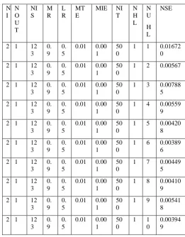
Table3.2: The values of the network parameters during testing
N I
N O U T
NI S
M R
L R
MT E
MIE NI T
N H L
N U
H L
NSE
2 1 12 3
0. 9
0. 5
0.01 0.00 1
50 0
1 1 0.01672 0
2 1 12 3
0. 9
0. 5
0.01 0.00 1
50 0
1 2 0.00567
2 1 12 3
0. 9
0. 5
0.01 0.00 1
50 0
1 3 0.00788 5
2 1 12 3
0. 9
0. 5
0.01 0.00 1
50 0
1 4 0.00559 9
2 1 12 3
0. 9
0. 5
0.01 0.00 1
50 0
1 5 0.00420 8
2 1 12 3
0. 9
0. 5
0.01 0.00 1
50 0
1 6 0.00389 6
2 1 12 3
0. 9
0. 5
0.01 0.00 1
50 0
1 7 0.00449 5
2 1 12 3
0. 9
0. 5
0.01 0.00 1
50 0
1 8 0.00410 9
2 1 12 3
0. 9
0. 5
0.01 0.00 1
50 0
1 9 0.00541 8
2 1 12 3
0. 9
0. 5
0.01 0.00 1
50 0
1 1 0
0.00394 9
[image:4.595.311.573.93.428.2]From the table 3.2, it can be known that, when the number of number units in the hidden layer (NUHL) is six, keeping other parameters fixed, the Normalized System Error is 0.003896. This error has been considered as the net error generated by the network during testing. Given below fig 3.2 is the graph between numbers of units in the hidden layer versus Normalized System Error (NSE) during training.
Fig 3.2: The graph between numbers of units in the hidden layer versus Normalized System Error (NSE) during
training.
The following table gives the performance of both of the networks (MLP VS SVR) with respect to their NSE values during training and testing.
0 0.005 0.01 0.015 0.02
1 2 3 4 5 6 7 8 9 10
NUHL Vs NSE
0 0.005 0.01 0.015 0.02
Table 3.3: The values of the network parameters during training and testing( For both of the networks)
Training
NI NOUT NIS NSE for
MLP
NSE for SVR
2 1 662 0.000517 0.0444
Testing
NI NOUT NIS NSE for
MLP
NSE for SVR
2 1 123 0.003896 0.0738
Experimental results show that MLP with back propagation algorithm performs much better than support vector regression model given the predefined set of variables as input to the above models. The MLP network outperforms SVR by 98.87% during training and 94.85% in testing phases of the networks which is clearly evident from the table 3.3.
Discussion and Conclusion:
The multi-layer perceptron neural network has been trained by back-propagation algorithm to predict the reliability of software along with the support vector regression model. It is essential to predict the reliability of software ,as more software’s that are being developed are error prone. Although, there are different models have been proposed for predicting the reliability of the software, the technology of neural networks will definitely be an added advantage given the larger the data set. The development of our model is a practical tool to predict the reliability of software given the predefined variables as input to the networks. As more data are generated, Both the systems improve in precision and can be widely employed in predicting the reliability of software in different environments. In Summary, we developed two network models, one is an MLP with back-propagation algorithm and the other is a Support Vector regression model to predict the reliability of software using the available information. The outcomes of both the models are consistent with the knowledge of the domain expert. Thus in this proposed research, the results support the reliability of the software by both of the networks and also gives an importance of understanding the impact of neural networks for finding the reliability of software.
References
[1] Liang T., Afzel, N. “On-line prediction of software reliability using an evolutionary” connectionist model”, Journal of Systems and Software, vol. 77,pp. 173–180, 2005.
[2] Hu Q., Xie M., and Ng S., Software Reliability Predictions using Artificial Neural Networks, Computational Intelligence in Reliability Engineering (SCI) 40, 197–222, 2007.
[3] Aljahdali, S. “Prediction of Software Reliability Using Neural Network and Fuzzy logic”, Ph.D. Dissertation presented to the faculty of College of Graduate Studies., Dept. of the Software Engineering and Info. System, George Mason University, Fairfax, Virginia, U.S.A, May 2003.
[4] Aljahdali, S., Sheta, A., and Rine, D., “Prediction of Software Reliability: A Comparison between regression and neural network non-parametric Models”,
Proceeding of the IEEE/ACS Conference, pp.470-471, 2000.
[5] Khoshgoftaar T.M., and Allen, E.B., “Logistic Regression Modeling of Software Quality”, International Journal of Reliability, Quality and Safety Engineering, 6(4), 1999.
[6] Stewart, W., “Collinearity and least squares regression”, Statistical Science, pp. 68-100, 1987.
[7] Aljahdali, S., Sheta, A., and Habib, M. "Software Reliability Analysis Using Parametric and Non- Parametric Methods”, Proceedings of the ISCA 18th
International Conference on Computers and their Application, March 26-28, 2003, pp. 63-66.
[8] Aljahdali, S., Sheta, A., and Rine, D., “Predicting Accumulated Faults in Software Using Radial Basis Function Network”, Proceedings of the ISCA 17th
International Conference on Computers and their Application, 4-6, April 2002, pp. 26-29.
[9] Narasinga Rao MR, Sridhar GR, Madhu K, Rao AA. A Clinical Decision Support System using Multilayer Perceptron Neural Network to Assess Well Being in Diabetes. J Assoc Physicians India 2009; 57:127–33. [10] Drucker.H, Burges C.j, Kaufman L, Smola A, Vapnik V,
Support Vector Regression Machines”, in Advances in Neural Information Processing Systems (1997), M.C.Mozer, M.I.Jordon, and T, Petsche(eds.),Vol.9,The MIT press,pp.155-161.
[11] Vapnik V, Golowich S.E, and Smola A, ‘Support vector method for function approximation, regression estimation and signal processing’, in Advances in Neural Information Processing Systems(1997), M.C.Mozer, M.I.Jordan, and T.petsche(eds.,),Vol.9, The MIT press, Cambridge, MA,pp.281-287.
[12] Scholkopf,B, Burges, C.,and Vapnik., V., ‘Incorporating invariances in support vector machines’, in Artificial Neural Networks—ICANN ’96, C.Vonder Malsburg,
W.von Seelen,J.Vorbuggen, and
B.Sendhoff(eds.,),Vol.1112 of Springer Lecture Notes in Computer Science, Springer- Verlag, Berlin,1996, pp.47-52.
[13] Mattera, D, Haykin.S., ‘ Support vector machines for dynamic reconstruction of a chaotic system’, in Advances in Kernel Methods- Support Vector Learning, B.Scholkpf, C.J.C.Burges, and A.J.Smola(eds.,), MIT Press, Cambridge,MA,1999,pp.211-242.
[14] Muller. K.R, Smola A.J, Ratsch. G, Kohlmorgan.J, and Vapnik.V., ‘Predicting time series with and support vector machines’, in Artificial Neural
Networks-ICANN’97, W.Gerstner,A.Germond,
M.Hasler,J.D.Nicoud,(eds.,), Springer Lecture Notes in Computer Science, Springer -Verlag, Berlin,1997, pp.999-1004,
[15] Stitson.M, Gammerman,A., Vapnik.V., Vovk.V., Watkins, C., and Weston, J., ‘Support vector regression with anova decomposition kernels’, in Advances in Kernels Methods-Support Vector Learning, B.Scholkopf, C.J.C.Burges, and A.J.Smola (eds.,), MIT Press, Cambridge, MA, 1997,pp.285-292. [16] M.A.H. Farquad, V.Ravi, S.Bapi Raju, “ Support Vector