6
I
January 2018
Position Verification and Identification of Primary
User Emulation (PUE) Attack in Cognitive Radio
Network
Miss. Priti Patil1, Prof. Mr. K.P.Paradeshi2.
¹P.G. Student, Department of Electronics Engineering, P.V.P.I.T Budhgaon, Sangli, India ²Associate Professor, Department of Electronics Engineering, P.V.P.I.T Budhgaon, Sangli , India
Abstract: Most of the people depend on the wireless spectrum in order to properly function. Wireless communication has many applications such as health services, national defense, security surveillance, financial transactions, and entertainment activities. These applications use the wireless spectrum. The use of wireless spectrum increases day by day, which results the wireless spectrum becomes overcrowded. Hence, most of the users cannot use the wireless spectrum efficiently. Cognitive radio is one of the fastest growing technologies in wireless communication. Cognitive radio is the solution to solve spectrum scarcity problem. In this network, unlicensed users share the spectrum of licensed user using spectrum sensing process. Spectrum sensing is important in transmission. When spectrum sensing process is disturbed, then the entire sensing process is disturbed, which is called as a primary user emulation attack. This attack is solved by using a localization method that is time-difference-of-arrival (TDOA).TDOA (Time Difference of Arrival) is simplest method for positioning. It is a kind of non-interactive positioning and uses the difference of arrival time, which is fit for the location verification of fixed transmitters.
Keywords: Cognitive radio network, primary user emulation attack, time difference of arrival, primary user, secondary user
I. INTRODUCTION
The use of wireless technology has increased day by day. Wi-Fi, WI-MAX, GSM, etc is popularly used by every person. Each of these wireless networks is carrying multiple communications. In the last 15 years, the percentages of people using the internet have increased most. Hence, radio spectrum becomes overcrowded.
The radio frequency spectrum is a sparse natural resource and its efficient use is the most importance. Satellite, mobile and fixed broadcast uses licensed spectrum bands to avoid harmful interference between different networks to affect the user. Most of the spectrum band has remained idle. Therefore, utilization of a spectrum band must be improved to meet the requirement of the spectrum. Spectrum is allocated only licensed users (primary users) are allowed use the spectrum band. A band of the spectrum is permanently allocated to users. These users are known as a licensed user. Most of the time licensed user does not use spectrum for communication. At that time spectrum remains idle. Therefore, frequency bands are simply wasted. According to new policy of FCC is to open up the licensed band to unlicensed users (secondary users) while no interference with licensed users [3].
Hence cognitive radio (CR), which enables opportunistic access to the spectrum, has emerged as the key technology. A CR is an intelligent wireless communication system, aware of its surrounding environment, and it adapts its internal parameters to achieve reliable and efficient communications [12]. These new networks have many applications, such as the cognitive use of the TV white space spectrum or making secure calls in emergency situations.
In cognitive radio network, there are two types of user primary user (PU), those who are licensed user and secondary user (SU), those who are unlicensed user. Primary user has the first priority to access the spectrum. When primary user is not active then secondary user uses that spectrum, as soon as primary user is becoming active, the Secondary user has to leave the channel for use by the PU. Since the Cognitive Radio (CR) provides the opportunity of spectrum usage only in the absence of the PU.
Figure.1. Representation of spectrum holes
A. Characteristics of cognitive radio are described as follows 1) Cognitive capability and reconfigurability
a) Cognitive Capability: It makes these devices to sense the information from its radio environment. Through this capability, the portions of the spectrum that are unused at a specific time or location can be identified. Consequently, the best spectrum and appropriate operating parameters can be selected.
b) Reconfigurability: It enables the radio to be dynamically programmed according to the radio environment. More specifically, the cognitive radio can be programmed to transmit and receive on different frequencies and to use different transmission access technologies.
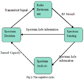
B. Cognitive radio mechanism is described as follows: 1) Cognitive Cycle Mechanism:
a) Spectrum sensing is one of the important mechanisms in cognitive radio. All SUs senses the spectrum bands, and captures the information, and then detects the spectrum holes.
b) Spectrum analysis is process that based on available information of spectrum holes that is feedback from spectrum sensing. It analyzes various channel and network characteristics for each spectrum hole and later provides this analysis to spectrum decision process.
Fig 2: The cognitive cycle.
II. LITERATURE REVIEW
This paper describes concept of cognitive radio and detection of spectrum holes. Spectrum hole is band of frequencies assigned to primary user, but, at particular time the band is not being utilized by that user. This paper also describes different types of spectrum hole [12].
This paper describes the details of primary user emulation attack (PUE). Primary user emulation (PUE) attack can be classified in two ways first is selfish attack and second is malicious attack. And this paper also presents a new transmitter verification procedure for spectrum sensing. Transmitter verification procedure is the estimation or verification of location of a signal’s origin. Cognitive radio continuously sense spectrum to check available channel [11].
This paper proposes a different approach to secure positioning that depends on the set of covert base station (CBS). Covert base station used for secure positioning. By the covert base station, base stations are those whose positions are not known to the attacker at the time of execution of secure positioning. For this some protocols are present in this paper [10].
This paper proposes a transmitter verification scheme, called localization based defense (Loc-Def). This scheme utilizes both signal characteristics and position of the signal transmitter to verify primary signal transmitter. Non-interactive localization scheme is introduced to detect PUE attacks [9].
III. PRIMARY USER EMULATION (PUE) ATTACK
The secondary user (SU) must have the ability of recognizing the primary user(PU) from SU signals. Some of the secondary users behave in bad ways and pretend itself as primary user to access the spectrum. Hence spectrum sensing process is corrupted is called as primary user emulation attack (PUEA).
Fig. 3 Representation of usual activity of secondary user sensing and transmission slot.
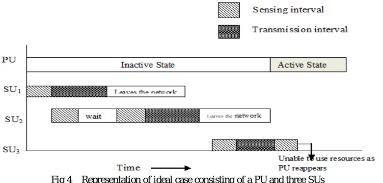
Fig. 3 shows the simple scenario of secondary user sensing and transmission interval. Fig. 4 consists of one primary user and three secondary users. Initially primary user is in inactive state. When primary user is inactive, SU1 arrives and perform sensing to check
for availability of bandwidth. After sensing SU1 finds the network to be available and transmits. Once SU1 is transmitting SU2
arrives and senses the availability of networks and finds network to be unavailable hence enters into wait state. In meanwhile SU1
finishes its transmission and leaves the network deliberately. Again SU2 senses the network and finds the network available and then
enter into transmission state. When SU2 finishes its transmission it leaves the network. Then SU3 comes and checks the availability
of network if network is available then it goes into transmission state. After completion of first transmission SU3 has some more
data to send for transmission hence it again senses the network to check the reappearance of PU and SU3
[image:5.612.115.505.416.603.2]finds PU to be active therefore SU3 has to leave the network. Because PU has the high priority.
Fig 4 Representation of ideal case consisting of a PU and three SUs
Now let assume an attack scenario where malicious SU named as SUm emulates all characteristic of PU and behave as PU. SUm
makes network unavailable for others SUs. Fig. 5 shows that SU1 comes and senses the network to check the availability of
bandwidth. Based on sensing result it transmits and leaves the network. While SU1 was transmitting, SU2 come and performed
sensing and entered into wait state. As soon as SU1 leaves the network, SUmemulates the characteristics of PU and pretends itself as
PU. SU2 senses again the network but malicious SU is pretending to be PU thus making SU2 to enter in other wait state. Ultimately
SU2 leaves the network without transmission. This phenomenon is called as Primary User Emulation Attack.
Fig 5 Representation of attack scenario by malicious SU making network resources unavailable.
If the PUE attack is successful then cognitive radio technology is unable to provide access to unlicensed users whenever the spectrum is vacant.
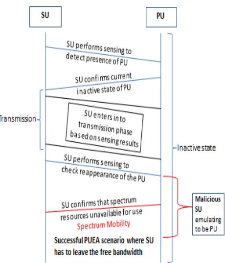
Fig. 6 shows the attack in more detail. Fig. 6 shows that SU perform sensing to detect the presence of PU. Based on sensing result SU confirms that PU is in inactive state. Therefore SU enters into transmission state. After completion of transmission SU again senses the network to check reappearance of PU i.e. PU is active because of emulation of malicious of SU. The result is spectrum mobility i.e. the SU has to vacate the spectrum resource currently underutilization.
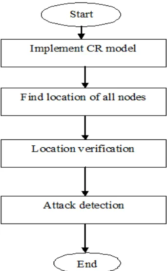
[image:6.612.212.442.442.711.2]IV. PROPOSED WORK
[image:7.612.222.393.146.423.2]To overcome the PUE attack, a transmitter verification scheme based on position verification is proposed. Several localization schemes have been proposed one of them is TDOA. TDOA is suitable in CRN because it utilize the difference between the arrival times of pulse.
Fig 7 Block Diagram of Proposed System
A. Localization of TDOA
TDOA (Time Difference of Arrival) is simple method for positioning. It is a kind of non-interactive positioning and uses the difference of arrival time, which is fit for the location verification of fixed transmitters.
Time Difference of Arrival is technique for locating sources near a microphone array. By exploiting thedifferences in the arrival time of the sound to the microphones, TDOA locates the source of the sound.
Let (xm ,ym, zm) be the coordinates of M microphone. Let (x,y,z) be unknown coordinates of sources. Let Tm be the time of transit from sources to microphone m. Let v be the speed of sound. Let Ɒm=vTmbe the distance between the source and the microphone m. Let Ʈm = Tm- t1 be the difference in transit time between microphone m and microphone 1.
Note that Ʈm=Τm –Τ1
Implies υ Ʈm=υΤm- υΤ1=Ɒm – Ɒ1 And therefore Ɒm2=(υƮm+Ɒ1)2=υ2Ʈm2+2υƮm+Ɒ12
We move everything over to get
0=υƮm+2Ɒ1+(Ɒ12–Ɒm2)/υƮm (1)
for m = 2,3,…,M. We now subtract 0=υƮm+2R1+(Ɒ12–Ɒ22)/υƮmfrom the above equation for m = 3,4,…,M. We then get the set of
equations
0= υƮm – υƮ2 + (Ɒ12–Ɒm2)/υƮm– (Ɒ12–Ɒ22)/υƮ2
for m = 3,4,..,M. We then substitute
Ɒm=[(xm–x)2+(ym–y)2+(zm–z)2]1/2 into the above equations to get
for m = 3, 4,…,M. Therefore
Ɒ12 - Ɒm2 = x12 + y12 + z12– xm2 – ym2–zm2–2x1x– 2y1y– 2z1z+2xmx+2ymy + 2zmz for m = 2,3,…,M. We now solve substitute the above result into Equation (1) to get
0=υƮm –υƮ2 +
Ʈ + (x1
2
+ y12 + z12– xm2 – ym2– zm2–2x1x– 2y1y – 2z1z +2xmx +2ymy + 2zmz)
–
Ʈ (x1
2
+ y12 + z12– x22 – y22– z22–2x1x– 2y1y – 2z1z +2x2x +2y2y + 2z2z)
for m = 3,4,…,M. We rewrite the above equation more succinctly as 0= Sm+ Amx+ Bmy + Cmz
Am =
Ʈ (–2x1 + 2xm) –Ʈ (2x2 – 2x1)
Bm=
Ʈ (–2y1 + 2ym) – Ʈ (2y2 – 2y1)
Cm =
Ʈ (–2z1 + 2zm) – Ʈ (2z2 – 2z1)
Sm= υƮm –υƮ2 +
Ʈ (x1
2
+ y12+ z12+ xm2– ym2– zm2) –
Ʈ (x1
2
+ y12+ z12+ x22– y22– z22)
for m = 3,4,..,M. We rewrite the above set of M - 2 equations into matrix form to get
3 3 3
4 4 4 =
− 3
− 4
−
Moore-Penrose pseudoinverse of matrix can be applied to both sides to calculate x,y,z values.Note that the yields a solution only when M >= 5. In other words, you need 5 or more microphones.
V. PERFORMANCE PARAMETER
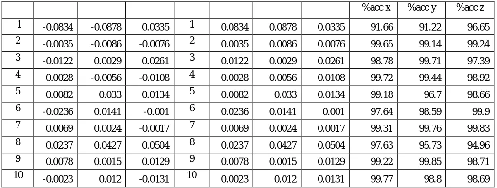
[image:8.612.47.502.64.318.2]Following table shows the accuracy of location using TDOA method. Proposed model is simulated using 10 nodes which are defined in terms of (x,y,z). True values are randomly generated. Proposed scheme calculates estimated values using TDOA method. Accuracy of proposed system is calculated using true value and estimated value of node. This model is simulated with five different sets of location data and results are calculated and averaged which are given as follows,
Table 1: True and estimated position of 10 nodes
Set 1 TRUE VALUES ESTIMATED VALUES
x y z X Y Z
1 13.2676 3.9607 1.9426 1 13.2861 3.969 1.9392
2 -13.9885 -38.7237 6.342 2 -13.9852 -38.708 6.3349
3 46.4027 10.2028 8.7749 3 46.3928 10.1978 8.7849
4 1.8571 -18.9873 15.904 4 1.8601 -18.9847 15.9068
5 -9.3243 0.6005 8.9117 5 -9.3396 0.6035 8.9207
6 -8.1614 -31.2681 15.0937 6 -8.1655 -31.2839 15.0784
7 -5.8996 -12.4767 13.102 7 -5.9086 -12.4958 13.098
8 5.9619 5.5283 9.9673 8 5.9393 5.5038 9.9401
9 -25.8109 40.4545 11.7054 9 -25.8058 40.4448 11.702
10 0.0891 -11.1902 5.1019 10 0.0872 -11.1622 5.0811
Table2: Percentage accuracy of 10 nodes
(Difference between true and estimated)Conversion of -veval in +ve
%acc x %acc y %acc z
1 -0.0185 -0.0083 0.0034 1 0.0185 0.0083 0.0034 98.15 99.17 99.66
2 -0.0033 -0.0155 0.0071 2 0.0033 0.0155 0.0071 99.67 98.45 99.29
3 0.0099 0.005 -0.01 3 0.0099 0.005 0.01 99.01 99.5 99
5 0.0153 -0.003 -0.009 5 0.0153 0.003 0.009 98.47 99.7 99.1
6 0.0041 0.0158 0.0153 6 0.0041 0.0158 0.0153 99.59 98.42 98.47
7 0.009 0.0191 0.004 7 0.009 0.0191 0.004 99.1 98.09 99.6
8 0.0226 0.0245 0.0272 8 0.0226 0.0245 0.0272 97.74 97.55 97.28
9 -0.0051 0.0097 0.0034 9 0.0051 0.0097 0.0034 99.49 99.03 99.66
10 0.0019 -0.028 0.0208 10 0.0019 0.028 0.0208 99.81 97.2 97.92
Table3: True and estimated position of 10 nodes
Set 2 TRUE VALUES ESTIMATED VALUES
x y z X Y Z
1 -10.4667 4.4749 6.222 1 -10.4258 4.4546 6.2304
2 -41.8005 19.6033 3.6963 2 -41.8193 19.6131 3.6963
3 44.8783 -5.4715 8.7774 3 44.8937 -5.7439 8.7787
4 -0.2814 5.5488 8.7774 4 -0.2794 5.4784 8.1292
5 -2.28 29.6573 12.0569 5 -2.2814 29.6534 12.0603
6 6.2797 35.0019 2.3484 6 6.2807 35.0145 2.3207
7 -6.2127 13.4701 8.4833 7 -6.2104 13.4735 8.4823
8 21.8147 12.9968 5.2496 8 21.815 12.9957 5.2439
9 39.3776 7.3119 18.5771 9 39.3822 7.3134 18.5805
10 -36.4231 2.6113 11.5705 10 -36.4241 2.6122 11.5894
Table4: Percentage accuracy of 10 nodes
(Difference between true and estimated)Conversion of -veval in +ve
%acc x %acc y %acc z 1 -0.0409 0.0203 -0.0084 1 0.0409 0.0203 0.0084 95.91 97.97 99.16 2 0.0188 -0.0098 0 2 0.0188 0.0098 0 98.12 99.02 100 3 -0.0154 0.2724 -0.0013 3 0.0154 0.2724 0.0013 98.46 72.76 99.87 4 -0.002 0.0704 0.6482 4 0.002 0.0704 0.6482 99.8 92.96 35.18 5 0.0014 0.0039 -0.0034 5 0.0014 0.0039 0.0034 99.86 99.61 99.66 6 -0.001 -0.0126 0.0277 6 0.001 0.0126 0.0277 99.9 98.74 97.23 7 -0.0023 -0.0034 0.001 7 0.0023 0.0034 0.001 99.77 99.66 99.9 8 -0.0003 0.0011 0.0057 8 0.0003 0.0011 0.0057 99.97 99.89 99.43 9 -0.0046 -0.0015 -0.0034 9 0.0046 0.0015 0.0034 99.54 99.85 99.66 10 0.001 -0.0009 -0.0189 10 0.001 0.0009 0.0189 99.9 99.91 98.11
Table5: True and estimated position of 10 nodes
Set 3 TRUE VALUES ESTIMATED VALUES
x y z X Y Z
1 -21.2762 2.4136 2.4122 1 -21.277 2.4135 2.4462
2 4.3936 29.1461 7.6924 2 4.3904 29.1384 7.7
3 -0.3308 29.1474 5.8088 3 -0.3322 29.1583 5.7956
4 -2.9579 30.7124 16.4875 4 -2.9563 30.7247 16.4901
5 -6.0818 -48.7553 6.8775 5 -6.0784 -48.7282 6.8789
6 22.7604 18.2978 18.1262 6 22.7649 18.2971 18.1308
7 18.1651 -40.0563 5.2146 7 18.1658 -40.0625 5.1988
8 29.421 4.1896 8.5052 8 29.4199 4.1902 8.4996
9 8.2546 13.2794 3.5753 9 8.257 13.2812 3.5797
Table6: Percentage accuracy of 10 nodes (Difference between true and estimated)Conversion of -veval in +ve
%acc x %acc y %acc z
1 0.0008 0.0001 -0.034 1 0.0008 0.0001 0.034 99.92 99.99 96.6
2 0.0032 0.0077 -0.0076 2 0.0032 0.0077 0.0076 99.68 99.23 99.24
3 0.0014 -0.0109 0.0132 3 0.0014 0.0109 0.0132 99.86 98.91 98.68
4 -0.0016 -0.0123 -0.0026 4 0.0016 0.0123 0.0026 99.84 98.77 99.74
5 -0.0034 -0.0271 -0.0014 5 0.0034 0.0271 0.0014 99.66 97.29 99.86
6 -0.0045 0.0007 -0.0046 6 0.0045 0.0007 0.0046 99.55 99.93 99.54
7 -0.0007 0.0062 0.0158 7 0.0007 0.0062 0.0158 99.93 99.38 98.42
8 0.0011 -0.0006 0.0056 8 0.0011 0.0006 0.0056 99.89 99.94 99.44
9 -0.0024 -0.0018 -0.0044 9 0.0024 0.0018 0.0044 99.76 99.82 99.56
10 -0.0286 -0.0209 -0.0257 10 0.0286 0.0209 0.0257 97.14 97.91 97.43
Table7:True and estimated position of 10 nodes
Set 4 TRUE VALUES ESTIMATED VALUES
x y z X Y Z
1 -10.7763 -33.0868 12.7706 1 -10.7909 -33.1218 12.7517
2 1.5256 0.704 6.392 2 1.3851 0.6402 6.2623
3 -14.9959 -21.9013 8.1524 3 -14.9943 -21.9001 8.1559
4 -8.0973 -40.1915 19.373 4 -8.1026 -40.2121 19.3571
5 -12.0827 23.66 2.1126 5 -12.0808 23.6594 2.0848
6 5.4981 -30.0491 8.4691 6 5.4961 -30.0443 8.4493
7 -0.4691 4.5169 3.0731 7 -0.4703 4.5247 3.09
8 -13.0664 5.1653 10.5429 8 -13.1057 5.1812 10.5743
9 16.2101 -16.1346 10.361 9 16.2118 -16.1338 10.372
10 -30.5945 -35.917 19.1539 10 -30.5936 -35.917 19.1375
Table8: Percentage accuracy of 10 nodes
(Difference between true and estimated)Conversion of -veval in +ve
%acc x %acc y %acc z
1 0.0146 0.035 0.0189 1 0.0146 0.035 0.0189 98.54 96.5 98.11
2
0.1405 0.0638 0.1297 2 0.1405 0.0638 0.1297 85.95 93.62 87.03
3 -0.0016 -0.0012 -0.0035 3 0.0016 0.0012 0.0035 99.84 99.88 99.65
4 0.0053 0.0206 0.0159 4 0.0053 0.0206 0.0159 99.47 97.94 98.41
5
-0.0019 0.0006 0.0278 5 0.0019 0.0006 0.0278 99.81 99.94 97.22
6
0.002 -0.0048 0.0198 6 0.002 0.0048 0.0198 99.8 99.52 98.02
7 0.0012 -0.0078 -0.0169 7 0.0012 0.0078 0.0169 99.88 99.22 98.31
8
0.0393 -0.0159 -0.0314 8 0.0393 0.0159 0.0314 96.07 98.41 96.86
9
-0.0017 -0.0008 -0.011 9 0.0017 0.0008 0.011 99.83 99.92 98.9
Table9: True and estimated position of 10 nodes Set 5 TRUE VALUESESTIMATED VALUES
x y z X Y Z
1 -1.4083 -1.6015 5.6373 1 -1.3249 -1.5137 5.6038
2 -9.0962 -25.3471 9.9823 2 -9.0927 -25.3385 9.9899
3 -25.2167 9.0458 2.4786 3 -25.2045 9.0429 2.4525
4 14.7823 -19.5604 17.4785 4 14.7795 -19.5548 17.4893
5 3.4874 13.057 11.2996 5 3.4792 13.024 11.2862
6 -27.7627 15.9446 4.1195 6 -27.7391 15.9305 4.1205
7
41.2333 23.3721 2.1142 7 41.2264 23.3697 2.1159
8 3.559 6.146 12.4192 8 3.5353 6.1033 12.3688
9 27.1635 9.2197 18.624 9 27.1557 9.2182 18.6111
10
[image:11.612.51.562.344.538.2]-2.7805 -36.3268 1.2681 10 -2.7782 -36.3388 1.2812
Table 10: Percentage accuracy of 10 nodes (Difference between true and estimated)Conversion of -veval in +ve
%acc x %acc y %acc z
1 -0.0834 -0.0878 0.0335 1 0.0834 0.0878 0.0335 91.66 91.22 96.65
2 -0.0035 -0.0086 -0.0076 2 0.0035 0.0086 0.0076 99.65 99.14 99.24
3 -0.0122 0.0029 0.0261 3 0.0122 0.0029 0.0261 98.78 99.71 97.39
4 0.0028 -0.0056 -0.0108 4 0.0028 0.0056 0.0108 99.72 99.44 98.92
5 0.0082 0.033 0.0134 5 0.0082 0.033 0.0134 99.18 96.7 98.66
6 -0.0236 0.0141 -0.001 6 0.0236 0.0141 0.001 97.64 98.59 99.9
7 0.0069 0.0024 -0.0017 7 0.0069 0.0024 0.0017 99.31 99.76 99.83
8 0.0237 0.0427 0.0504 8 0.0237 0.0427 0.0504 97.63 95.73 94.96
9 0.0078 0.0015 0.0129 9 0.0078 0.0015 0.0129 99.22 99.85 98.71
10 -0.0023 0.012 -0.0131 10 0.0023 0.012 0.0131 99.77 98.8 98.69
Table11: Average value of x position of all nodes.
Set 1 Set 2 Set 3 Set 4 Set 5
% Accuracy x % Accuracy x % Accuracy x % Accuracy x % Accuracy x Average
1 98.15 95.91 99.92 98.54 91.66
2 99.67 98.12 99.68 85.95 99.65
3 99.01 98.46 99.86 99.84 98.78
4 99.7 99.8 99.84 99.47 99.72
5 98.47 99.86 99.66 99.81 99.18
6 99.59 99.9 99.55 99.8 97.64
7 99.1 99.77 99.93 99.88 99.31
8 97.74 99.97 99.89 96.07 97.63
9 99.49 99.5 99.76 99.83 99.22
Table12: Average value of y position of all nodes.
Set 1 Set 2 Set 3 Set 4 Set 5
% Accuracy y % Accuracy y % Accuracy y % Accuracy y % Accuracy y Average
1 99.17 97.97 99.99 96.5 91.22
2 98.45 99.02 99.23 93.62 99.14
3 99.5 72.76 98.91 99.88 99.71
4 99.74 92.96 98.77 97.94 99.44
5 99.7 99.61 97.29 99.94 96.7
6 98.42 98.74 99.93 99.52 98.59
7 98.09 99.66 99.38 99.22 99.76
8 97.55 99.89 99.94 98.41 95.73
9 99.03 99.85 99.82 99.92 99.85
10 97.2 99.91 97.91 100 98.8
Table13: Average value of z position of all nodes.
Set 1 Set 2 Set 3 Set 4 Set 5
% Accuracy z % Accuracy z % Accuracy z % Accuracy z % Accuracy z Average
1
99.66 99.16 96.6 98.11 96.65
2
99.29 100 99.24 87.03 99.24
3
99 99.87 98.68 99.65 97.39
4
99.72 35.18 99.74 98.41 98.92
5
99.1 99.66 99.86 97.22 98.66
6
98.47 97.23 99.54 98.02 99.9
7
99.6 99.9 98.42 98.31 99.83
8
97.28 99.43 99.44 96.86 94.96
9
99.66 99.66 99.56 98.9 98.71
10
VI. RESULT
[image:13.612.152.480.132.397.2]Figure 8 shows that the representation of 2D GUI. First graph is true position graph and second graph is eastimated position graph. Using TDOA algorithm we have to match both values. In following figure true position and estimated position values are not matched. Hence it might be chances of attack.
Fig. 8 Representation of 2D GUI
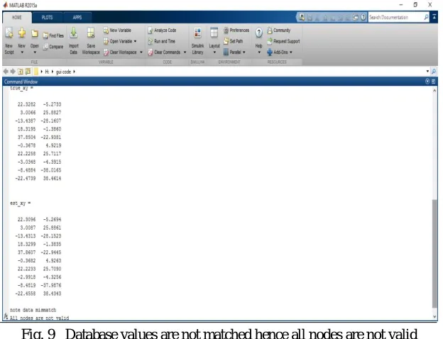
[image:13.612.161.473.443.682.2]Fig. 9 shows the actual database values of the node. True position values and estimated position values are not matched. From these values we come to know that attack is happened in cognitive radio network. Furthere communication is not happen. Attacker uses the bandwidth for bad purpose. Hence all nodes are not valid.
Fig. 9 Database values are not matched hence all nodes are not valid
Fig. 10 Database values are matched hence all nodes are valid
Fig. 11 shows that the representation of 3D GUI. First graph is true position graph and second graph is eastimated position graph. Using TDOA algorithm we have to match both values. In following figure true position and estimated position values are not matched. Hence it might be chances of attack.
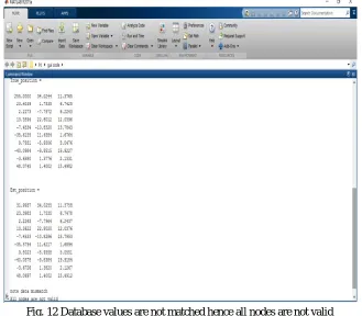
Fig. 12 shows the actual database values of the node. True position values and estimated position values are not matched. From these values we come to know that attack is happened in cognitive radio network. Furthere communication is not happen. Attacker uses the bandwidth for bad purpose. Hence all nodes are not valid.
[image:15.612.131.505.436.717.2]Fig. 12 Database values are not matched hence all nodes are not valid
Fig. 13 shows the database values are matched. True position and estimated position values are matched. Hence attack is not happen in cognitive radio netwwork. All nodes are valid hence further communication will take place properly.
VII. CONCLUSION
CRN is based on spectrum sensing mechanism. It defines spectrum holes in the spectrum which are unused by primary user. An attacker behaves as primary user and performs the PUE attack. The problem of PUEA can be solved using TDOA method. TDOA method finds the position of attacker. The proposed method has been implemented using MATLAB. A result shows that this method can improve the localization accuracy which strengths the ability of PUE attack.
REFERENCES
[1] W. R. Ghanem, M.Shokair and M. I. Desouky, “An improved primary user emulation attack detection in cognitive radio network based on Firefly Optimization Algorithm”, 33rd National Radio Conference (NRSC 2016), Feb 22-25,2016 pp. 178-187.
[2] F. Jin, V.Vardharajan and U. Tupakula, “Improved detection of primary user emulation attack in cognitive radio network”, International Telecommunication Network and Application Conference (ITNAC), Nov,2015, pp. 274-279.
[3] K. K. Chaunhan and A. K. Singh Sanger, “Survey of security threads and Attacks in cognitive radio networks”, International Conference on Electronics and communication system (ICECS), Feb,2014, pp. 01-05.
[4] M. Dang, Z. Zhao and H. Zhang, “Optimal Cooperative Detection Primary User Emulation Attacks in Distributed Cognitive Radio Networks”, 8th International Conference on Communication and Networking in China(CHINACOM), Aug,2013, pp. 368-373.
[5] Bilal Nqvi, Imran Rashid, Faisal Riaz, Baber Aslam, “Primary User Emulation Attack and their mitigation strategies: A survey”, 2nd National Conference on
Information Assurance(NCIA),2013
[6] C. Chen, H. Cheng and Y. Yao, “Cooperative Spectrum Sensing in Cognitive Radio Network in the presence of Primary User Emulation Attack”, IEEE Transactions on Wireless Communication, Vol 10, no. 7, July,2011, pp. 2135-2141.
[7] D. Pu, Y. Shi, A. V. VIlyashenko and A. M. Wyglinski, “Detecting Primary User Emulation attacks in Cognitive Radio Networks”, In Proceedings of the IEEE Global Telecommunication Conference(GLOBECOM)IEEE, Dec 2011, pp. 01-05.
[8] X. Ding, X. Gong and R. Wu, “The study onrelated algorithm of TDOA positioning,” Modern ElectronicTechnology, No.1, 2009.
[9] R.Che, J. Park and J. Reed, “Defense against primary user emulation attacks in cognitive radio networks,” IEEE Journal on Selected Areas in Communications, vol. 26, no.1, Jan. 2008, pp. 25-37.
[10] S. Capkun, M. Cagalj and M. Srivastava, “Secure localization with hidden and mobile base stations,” proc. IEEE Infocom, Apr. 2006.
[11] R Chen nd J Park, “Ensuring Trustworthy Spectrum Sensing in Cognitive Radio Network”,1st IEEE workshop onNetworkingTechnologies for Software
Defined Radio, SDR ’06. 25-27sept. 2006 Pages(s):110-119.
[12] S. Haykin, “Cognitive radio: brain-empowered wirelesscommunications,” IEEE Journal on Selected Areas inCommunications, Vol 23 (2), Feb. 2005, pp.201-220.
[13] Federal Communication Commission, “Notice for Proposed Rulemaking (NPRM 03-322): Facilitating Opportunities for Flexible Efficient and Reliable Spectrum Use EmployingCognitive Radio Technologies”, ET Docket, No.03-108, Dec.2003.