ISSN: 1992-8645 www.jatit.org E-ISSN: 1817-3195
STUDY OF CONVEX QUADRATIC BILEVEL
PROGRAMMING PROBLEM ORTHOGONAL GENETIC
ALGORITHM
1XIAOYUN YUE, 2GUANCHEN ZHOU, 3JINFENG LV
1
Hebei Normal University of Science and Technology, Qinhuangdao 066004, China 2
Qinggong College, Hebei United University, Tangshan 063009, Hebei, China 3 Hebei Normal University of Science and Technology, Qinhuangdao 066004, China
ABSTRACT
This paper introduces the research status of convex quadratic bilevel programming at present firstly. Secondly, it analyzes the problem of convex quadratic bilevel programming models, concepts and properties. On this basis, using the optimality conditions of KKT, the problem will be transformed into a single complementary slackness relaxation problem. To solve this problem, we propose an orthogonal genetic algorithm by the KKT multipliers for the introduction of 0-1 binary encoding. The paper in the wood orthogonal genetic algorithm designs of hybrid operators to increase the factor analysis. We carry out algorithm convergence analysis and numerical experiments. Finally, Numerical results show that the proposed orthogonal genetic algorithm is effective and reasonable by giving a example.
Keywords: Convex Quadratic Bilevel Programming, Orthogonal Genetic Algorithm, KKT Conditions, Global Optimization
1. INTRODUCTION
In optimization problems, convex programming has much good behavior, the use of these properties made many excellent algorithms. Accordingly, the convex bilevel programming problem is the nonlinear bilevel programming problem which has special structure and properties, because of its hierarchical structure; in fact it belongs to a class of no convex global optimization problems.
Convex quadratic bilevel programming problem is a special class of nonlinear bilevel programming problems, because all of its objective function is convex quadratic function, all the constraint functions are linear, so it belongs to the convex layers planning issues. Convex quadratic bilevel programming has some good properties [1-3]. Such as the induction field is piecewise linear continuous; solution of the problem is convex set: the lower bound to meet the specifications of planning conditions, KKT optimality conditions are necessary and sufficient conditions: there is the global optimal solution.
Although the convex quadratic bilevel programming problem has some good properties, due to constraints of the nested nature, in essence, it is a non-convex programming. For such difficult NP problem to solve the global optimal solution is
very difficult. So far, solving quadratic bilevel programming problem, particularly for large scale problems, there is only a few of effective algorithm. We use convex quadratic bilevel programming method for solving common problems: KKT conditions for using the two-tier planning problem into an equivalent single-layer complementary relaxation problem, and then use the method based on branch and bound to solve. a document [1,2], that is, in this way.
In this paper, using KKT optimality conditions turn the original problem into a single complementary relaxation problem. KKT multipliers for the introduction of 0-1 binary encoding designed a complementary orthogonal genetic algorithm to solve the relaxation problem. Convex quadratic programming problem maybe has more feasible solution, so the paper in the wood orthogonal genetic algorithm designs of hybrid operators to increase the factor analysis.
2. MODELS, CONCEPTS AND
PROPERTIES OF CONVEX QUADRATIC BILEVEL PROGRAMMING PROBLEMSY
2.1Models and concepts
( )
[
]
k y x P Y x y xF T T
y
x
= , , min ,
[
]
+ + y x b aT, T(1a )
s.t. Ax+By≤r1 (1b)
( )
[
]
= y x Q Y x y xf T T
y , ,
min
[
]
+ y x D CT, T
(1c) 2
.
.t Cx Dy r
s + ≤ (1d)
, , , , , , ,
, 1 2
q p m n m n R r R r R d b R c a R y R
x∈ ∈ ∈ ∈ ∈ ∈
n p R
A∈ × ,B∈Rp×m,C∈Rq×n,D∈Rq×m,k∈R
. P,Q are n+m -dimensional positive definite matrixs.
Suppose
= 1 2 2 3 Q Q Q Q Q T , and n n n m m m R Q R Q R
Q1∈ × , 2∈ × , 3∈ × . So the problem (1) and the following problem (2) have the same optimal solution.
( )
[
]
( )
= − y x P Y x y xF T T
y
x 2 , 2
1 , min ,
[
]
+ y x b aT, T(2a
)
s.t. Ax+By≤r1 (2b)
( )
x y y Q y(
d Q x)
yf T T
y , 1 2 2
min = + +
−
(2c) 2
.
.t Cx Dy r
s + ≤ (2d)
Collections of relevant definitions are given below:
Binding domains of question (2):
( )
{
x,y :Ax+By≤r1,Cx+Dy≤r2}
= Ω
For eachx, the reasonable response set of lower:
( )
≤ + ∈= y:y argmin −f x,−y :Cx D−y r2 x
R
Induction field of issues (2) (or feasible region):
( ) ( )
( )
{
x y x y y R x}
IR= , : , ∈Ω, ∈
Definition 1: Called the optimal solution of
( ) ( )
∈ − IR y x y x F , : , minis the optimal solution for problem (2).
Assuming 1: Ωis non-bounded set, IRis also nonempty bounded.Because Ω is n+m
-dimensional positive definite matrix, so Q1 is m -dimensional positive definite matrix.
The lower plan of problem (2) is strictly convex quadratic programming, then for each given x, the lower plan has a unique optimal solution, the reasonable response set R
( )
x of the lower set is a single value. P is a positive definite matrix,( ) ( )
x y x y F , : ,−
is a quadratic strictly convex, by assumption 1, Global optimal solution of QBLPP must exist.
2.2Properties
Using KKT optimality conditions, turn the problem (2) into a single complementary relaxation problem [3,4,5]
( )
[
]
( )
[
]
+ = − y x b a y x P y x y xF T T T T
u y x , 2 , 2 1 , min , , (3a) 0 2 2 .
.t Q2x+ Q1y+d+D u=
s T (3b)
(
Cx+Dy+d+D u)
=0U T (3c)
2 1,Cx Dy r
r By
Ax+ ≤ + ≤ (3d)
( )
u diag Uu≥0, = (3e)
u is the q -dimensional vector of KKT multipliers, equation (3c) is called the complementarity condition, it is nonlinear.
when given the upper layer variable x , the problem (2) is the lower strictly convex quadratic programming planning, assuming that for fixed x, the optimal solution in the lower bound place to meet specifications, so KKT optimality conditions of lower programming problem is the necessary and sufficient condition [6], then the original problem (2) and problems (3) are equivalent. Existence of the complementarily condition (3c.), the problem (3) is a non-convex programming.
3. DESIGN OF THE CONVEX QUADRATIC
BILEVEL PROGRAMMING ALGORITHM
3.1.Chromosome codes
ISSN: 1992-8645 www.jatit.org E-ISSN: 1817-3195 problem (3), a KKT multiplier vector
) , , ,
(u1 u2 uq
u=
corresponds to a binary string chromosomes=(s1,s2,,sq), among them
) , , 2 , 1
(i q
si = equal to 0 or 1. For q
i=1,2,, , if si =0, then corresponds to the
ith -KKT multiplier ui =0 ; if si =1 , then corresponds to the ith-KKT multiplier ui >0.
For each i∈
{
1,2,,q}
, if si =0 , then corresponds to the ith-KKT multiplier ui =0, soi i
ix Dy r
C + ≤ 2 , if si =1, then corresponds to the
ith-KKT multiplier ui>0, so Cix+Diy=r2i. Thus, for each chromosome, the problem (4) can be simplified to a quadratic programming, and quadratic programming problems, whether the issue of size, can be easily solved using existing algorithms, such as interior point method, active set method , dual methods, trust region method [7, 8].
If the quadratic programming constraints incompatible or contradictory, it is no solution, then the corresponding chromosome is called feasible. If the quadratic programming problem solvable, then the corresponding chromosome is called feasible. For feasible chromosomes, by solving the corresponding quadratic programming problem, we can got the optimal solution ( , , )
∗ ∗ ∗
u y
x , The
objective function value ( , )
∗ ∗
y x
F is defined as
the possible fitness value of chromosomes. At this time, ( , )
∗ ∗
y
x is called a feasible solution.of the
original bilevel programming problem (2), on the not feasible chromosome providing the fitness value+∞.
Taking into account the evolution may be many feasible chromosomes. To be able to quickly identify parts of the chromosome is not feasible, using the following method screening.
If the problem has constraints Li ≤ yi ≤Ui , where Li and Ui are the lower bound and upper bound of the ithvariable i=1,2,,m, part of the infeasible chromosomes can be pre-determined.
For example, problem (6), by the
complementarily conditions
0 ) 5 . 0 ( 1
1 −y =
u , u2(y1−1.5)=0 and 5
. 1 5
.
0 ≤ y1≤ , we can see the chromosome is not
feasible which has the form as (11∗∗), where ∗ denotes can be taken by 0 or 1. By the complementarily
conditions u3(0.5− y2)=0 , u2(y1−1.5)=0 and 5
. 1 5
.
0 ≤ y2≤ , we can see the chromosome is not feasible which has the form as (∗∗11)
Let binary string (0110) is a chromosome of the problem (6), the corresponding quadratic programming problem is:
= 2 1 2 1 2 1 2 1 , , 2 0 0 0 0 2 0 0 0 0 2 0 0 0 0 2 ] , , , [ 2 1 ) , ( min y y x x y y x x y x F u y x − − + 2 1 2 1 ] 0 , 0 , 3 , 3 [ y y x x 0 ) ( 2 , 0 ) ( 2 . . 3 2 2 2 1 1 = − − = + − u x y u x y t s 0 , 0 , 0 5 . 0 , 0 5 . 1 3 2 2 1 ≥ ≥ = − = − u u y y
Solving the above quadratic programming, we know that chromosome (0110) is feasible, the
fitness value is −1 ,
(
x1,x2,y1,y2) (
= 1.5,0.5,1.5,0.5)
is a feasiblesolution of the two problems (5).
3.2.Initialization
Randomly generated the initial population and population size is Np , including the infeasible chromosome.. In order to avoid double counting the same fitness value of chromosomes, feasible and infeasible chromosomes were retained in two different lists. Then, check whether the chromosomes present in these two lists. If it appears in the list of feasible chromosome, it is not nessary to solve the corresponding quadratic programming solutions, and directly got its fitness value. If it appears in the list of infeasible chromosome, its fitness value is +∞
As algorithms 1, generating Np initial chromosomes to form the initial population.
Step1. Generating q -dimensional random vector γ =γ(γ1,,γi,γq) , γi∈(0,1) is a random number.
Step2. For everyi∈
{
1,2,,q}
, Ifγi <0.5, let0
= i
s ; otherwise si =1 , so that generate a
chromosome(s1,,si,sq)
Step3. Repeat the above two steps Np times, generating Np initial chromosomes to form the initial population.
Step4. By the boundary conditions, first screening out infeasible chromosome, and define its fitness value as
+
∞
Step5. Solve quadratic programming problem which chromosomes corresponds to. If some problem has no solution, the corresponding chromosome is not feasible, and their fitness value is defined as
+
∞
. If some quadratic programming problem solvable ( , , )∗ ∗ ∗
u y
x , the fitness of these
chromosomes are ( , )
∗ ∗
y x
F .
step6. Store the feasible and infeasible chromosomes in two different tables
3.3.Crossover Operator
Orthogonal experimental design as the crossover operator, making the hybrid produced by the orthogonal and uniform representation of future generations, and then through factor analysis, to find the best chromosome which is better than the parent.
Each chromosome has qgenes; every gene can be taken by 0 or 1. Insult genes as a factor, so the insult factor has two levels. So, here we use the two-level orthogonal table (2 )
1 −
N N
L . In the
experiment, according to length of chromosome string, select the appropriate two-level orthogonal table. Letq≤ N−1. If q= N−1. Directly got the standard two-level orthogonal (2 )
1 −
N N
L .
If q<N−1 , , use two-level orthogonal table
) 2 ( q
N
L .
Take the best chromosome as a level 1. Then by crossover probability pc , randomly select a chromosome different from the former as a level 2. Using these two chromosomes do two level orthogonal table (2 )
1 −
N N
L matrix experiment, and
produce N offspring chromosomes. Finally,
estimate the fitness value of the produced chromosomes.
Analyze feasible chromosome by factors analysis. Let Fi shows fitness value which is combination factors in the
ith
test results showed that combination factors (feasible chromosome), i∈{
1,2,,N}
. i is the corresponding indicators of feasible chromosome., take the kth level influence degree of he factor j asEkj, j=1,2,q,and k=1,2∑
∈⋅ =
N i
i i
kj F
E χ
(7) If the level of factor j is k in the ithtest,
1
= i
χ ; otherwise χi =0 . Problem (3) is the
minimize problem, if E1j <E2j , indicating that the level 1 of factor j is better than level 2, level 1, level 2, otherwise choose. All factors in a good level of choice, the inherited genetic parent of the new chromosome is better. To avoid unnecessary calculation, check whether the resulting chromosomes present in the two lists tables mentioned earlier. If chromosomes present in a table, then their fitness value can be known. If some other chromosome do not appear in the list, by solving the corresponding quadratic programming problem, and then calculate the fitness value of the feasible chromosomes. Infeasible chromosome fitness value is defined as+∞. Of course, they are also keeping in the corresponding table.
3.4. Selection operator
According to the fitness value, Arrangement the current generation chromosome, hybridization and mutational damage chromosomes, and then select the former Np chromosome as the next generation of population, and retain the best chromosome, of course there maybe infeasible chromosomes. Because their fitness value is +∞. So infeasible chromosome randly complement in the feasible chromosome, after reached Np , but it is also beneficial to keep the diversity of population.
3.5. Stopping criteria
ISSN: 1992-8645 www.jatit.org E-ISSN: 1817-3195
3.6. Algorithm convergence analysis
The lower level question (2) has q (limited) constraints, thus KKT multiplier vector u is the
qdimension, so it has q KKT multiplier. Each
KKT multiplier was equal to 0 or bigger than 0, then the KKT multiplier vector
u
has at most 2q entire combination. If it is non solution, then this chromosome is not feasible, this KKT multiplier vectoru
can be removed; If it has solution, this chromosome is feasible. Therefore through the feasible inspection, we can remove a part of KKT multiplier vector combination. Therefore the feasible chromosome isles than2q, Through the implicit enumeration limited a feasible chromosome (local optimal solution) to find global optimal solution of problem (l). Using similar to the standard genetic algorithm of Marko chain convergence theory, the algorithm probabilistic l convergence to the global optimal solution of question ( l)3.7. Numerical experiments
To verify the effectiveness of the method, select defend types second two layers to test, and compare the result with reference [9, 10].
Experiment parameter is used in test ;
population size Np,: for question1- 6, 8 and 9Np =8, for question 7 Np=12;for problem 12
16
= p
N
; interbreeding probability pc=0.8 . Mutation probability pm =0.2 . Maximum evolutionMaxG=5.
Use two levels orthogonal table: problem 1 and 6, use (2 )
3 4
L ; the problem 2- 5,8and 9, use
) 2 ( 6 8
L ; 'Question 7 use L8(26), Problems 10 use )
2 ( 12 16
L
Using MATLAB code that for every problem independently operating 30 times. For quadratic programming problem, invoked the optimal toolbox function "quadProg"of MATLAB solve quadratic programming.
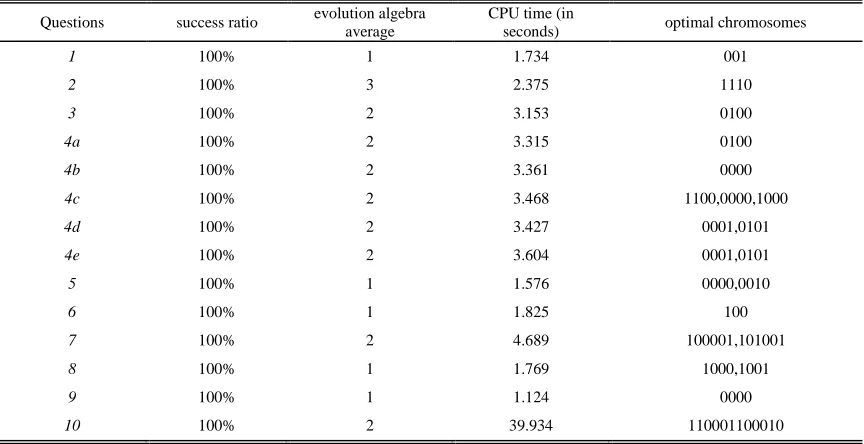
[image:5.612.91.523.423.645.2]For every problem, use different initial population, run 30 times, income statistical results see table 1, including the success ratio, average evolution algebra, average CPU time (in seconds) and unit: the optimal chromosomes.
Table: Independent Running 30 Times, All Statistical Results Of The Problems
Questions success ratio evolution algebra average
CPU time (in
seconds) optimal chromosomes
1 100% 1 1.734 001
2 100% 3 2.375 1110
3 100% 2 3.153 0100
4a 100% 2 3.315 0100
4b 100% 2 3.361 0000
4c 100% 2 3.468 1100,0000,1000
4d 100% 2 3.427 0001,0101
4e 100% 2 3.604 0001,0101
5 100% 1 1.576 0000,0010
6 100% 1 1.825 100
7 100% 2 4.689 100001,101001
8 100% 1 1.769 1000,1001
9 100% 1 1.124 0000
10 100% 2 39.934 110001100010
Success ratio is to point that the percentage in the operation of finding the optimal solution in 30 times. Let the algorithm of the optimal results and
Table 2:The Results Of The Results In The Reference
Questions
ResultS
)
,
(
x
y
F
(
x
,
y
)
f
(
x
,
y
)
1[106] (0.8462,0.7692,0) -2.0769 -0.5917
2[106] (0.6111,0.3889,
0,0,1.8333) 0.6389 1.6806
3[107] (25,5,10,5) 225 100
4a[108] (1.0316,3.0978,
2.5970,1.7929) -8.9172 -6.1370
4b[108] (0.2788,0.4748, 2.3438,1.0325) -7.5785 -0.5719
4c[108] (11.9344,38.8950,
2.9885,2.9895) -3.5 -2.2
4d[108] (2,0,2,0) -3.8 -2.1
4e[108] (-0.4,0.9,2,0) -3.95 -2
5[110] (0.5,0.6,0.5,0.5) -1 0
6[109] (10,10) 100 0
7[109] (1.8888,0.8888,0) -1.2098 7.6175
7[109] (1.8888,0.8888,0) -1.2098 7.6175
8[103] (1,0) 17 1
9[110] (0.75,0.75,0.76,0.78) -2.5 0
10[103] (7,3,12,18,0,
11,32,0) 6600 25, 29
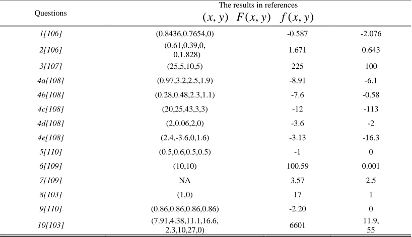
Table 3 :The results and comparison of the results in the reference
Questions
The results in references
)
,
(
x
y
F
(
x
,
y
)
f
(
x
,
y
)
1[106] (0.8436,0.7654,0) -0.587 -2.076
2[106] (0.61,0.39,0,
0,1.828) 1.671 0.643
3[107] (25,5,10,5) 225 100
4a[108] (0.97,3.2,2.5,1.9) -8.91 -6.1
4b[108] (0.28,0.48,2.3,1.1) -7.6 -0.58
4c[108] (20,25,43,3,3) -12 -113
4d[108] (2,0.06,2,0) -3.6 -2
4e[108] (2.4,-3.6,0,1.6) -3.13 -16.3
5[110] (0.5,0.6,0.5,0.5) -1 0
6[109] (10,10) 100.59 0.001
7[109] NA 3.57 2.5
8[103] (1,0) 17 1
9[110] (0.86,0.86,0.86,0.86) -2.20 0
10[103] (7.91,4.38,11.1,16.6,
2.3,10,27,0) 6601
11.9, 55
4. CONCLUSIONS
Two evolutionary algorithms for the discrete BLPP are presented. The discrete linear BLPP is firstly transformed into a 0-1 BLPP in which the lower level problem can be solved by the branch and bound algorithm, and then the problem is transformed into a single level 0-1 programming, which is solved by the orthogonal genetic algorithm. In addition, for the discrete nonlinear BLPP with discrete upper level variables and
continuous lower level variables, the lower level problem can be solved by the traditional optimization algorithms. This bilevel problem is then transformed into a single level discrete programming problem, which is solved by the hybrid evolutionary algorithm. Some numerical examples are used to test their performance. The simulation results show that two evolutionary algorithms are effective.
[image:6.612.104.513.341.577.2]ISSN: 1992-8645 www.jatit.org E-ISSN: 1817-3195 programming problem. For convex two layers
quadratic programming problem, based on equivalent transformation form of the KKT condition, puts forward a kind of orthogonal genetic algorithm. In the Algorithm, a hybrid orthogonal experiment design as will operator, By using orthogonal table generate multiple hybrid progenies, then using factor analysis to identify good factor levels in order to get a better offspring. By using two sites mutation, generate mutation operator. For KKT multipliers, introducing 0-1 coding method, complementary flabby problem can be transformed into a series of quadratic programming problem.
For the quadratic programming, by solving it, we can got the chromosome fitness value and a feasible solution of the former two layers programming problem. Using this strategy, we can effectively solve complementary droopy. Numerical experiments show that the orthogonal genetic algorithm is efficient and robust.
ACKNOWLEDGEMENTS
This work was supported by the Scientific Technology Research and Development Program Fund Project in Qinhuangdao city (No. 2012025A0 34)
REFERENCES:
[1] J.Bard, "Convex two-level optimization",
Mathematical Programming, Vol. 40, 1988, pp.15-27.
[2] J.Bard , J.Moore, "A branch and bound algorithm for the bilevel programming problem", SIAM Journal on Scientific Statistical Computing, Vol. 40, 1990, pp.281-292.
[3] T.Edmunds, J.Bard, "Algorithms for nonlinear bilevel mathematical programming", IEEE Trans. on Systems, Man,and Cybernetics, Vol. 21, 1991,pp. 83-89.
[4] Yuping Wang, Yong-Chang Jiao, Hong Li,"An evolutionary algorithm for solving nonlinear bilevel programming based on a new constraint-handing scheme", IEEE Trans.on Systems, Man and Cybernetics-Part C, Vol. 35,No 2, 2005, pp. 221-232.
[5] D.L.Zhu, Q.Xu,Z.Lin, "A homotopy method for solving bilevel programming problem",
Nonlinear Analysis, Vol. 57, No 2, 2004,pp. 917-928.
[6] S.Dempe, "First-Order Necessary Optimality Conditions for General Bilevel Programming Problems", Journal of Optimization Theory and Applications, Vol. 95, No 3, 1997,pp. 735-739. [7] N.P.Faísca, V.Dua, B.Rustem, "Parametric
global optimisation for bilevel programming",
Journal of Global Optimization, Vol. 38, 2007,pp.609-623.
[8] K.Deb, "An efficient constraint handing method for genetic algorithms", Computer Methods in Applied Mechanics and Engineering, Vol. 186,No 4, 2000, pp.311-338, [9] Thomas Weise, Raymond Chiong,
"Evolutionary Optimization: Pitfalls and Booby Traps", Journal of Computer Science & Technology,Vol. 18, No 5, 2012,pp.311-338. [10]I.A.Chaudhry, "Job shop scheduling problem
with alternative machines using genetic algorithms", Journal of Central South University, No 5, 2012, pp.368-382.
[11] Aimin Yang, Chunfeng Liu, Jincai Chang and Li Feng, “TOPSIS-Based Numerical Computation Methodology for Intuitionistic Fuzzy Multiple Attribute Decision Making”,
Information-an International Interdisciplinary Journal, Vol. 14,No.10 pp.3169-3174.
[12] Aimin Yang, Chunfeng Liu, Jincai Chang, Xiaoqiang Guo, “Research on Parallel LU Decomposition Method and It’s Applica tion in Circle Transportation”,Journal of Software, Vol 5, No.11,2010, pp.1250-1255.