ISSN: 1992-8645 www.jatit.org E-ISSN: 1817-3195
THE MIXTURE MODEL: COMBINING LEAST SQUARE
METHOD AND DENSITY BASED CLASS BOOST
ALGORITHM IN PRODUCING MISSING DATA AND
BETTER MODELS
LADAN MALAZIZI
Computer Engineering Department Islamic Azad University, Najafabad Branch
Esfahan, Iran
E-mail: [email protected]
ABSTRACT
The problem of missing values in data tables arises in almost all domains. With the volume of the information growing every day on the communication channels and the necessity of the integration of this data for data analysis and data mining, this reflects even more. In this paper with two step process first we recover missing values using Least Square method (LS) [1] then we use our own Density Based Class Boost Algorithm (DCBA) [2] in order to improve learner performance. In this process we model the data using Meta learner once when data tables have been cleaned (removing empty rows containing missing values), then when data has been recovered and lastly after application of The Mixture Model. In this paper our contributions are toward three issues: first the effect of data cleaning in the mean of losing data with missing cells in model performance, second the effect of Least Square method in data generation in such highly correlated features datasets and third the effect of the combination model in classifier performance.
Keywords:Least Square, Density Based Class Boost, Missing data recovery
1.INTRODUCTION
The subject of missing values recovery in databases has long been studied and discussed in different domains. This is a biggest problem of data storage and processing. Incomplete data reduces quality and reliability. But the significance of the missing data and its effect on data mining is not always clear in final analysis. In some domains when the data is processed, the incomplete data is simply ignored, deleted at data cleaning stage or not considered in analysis.
Following our previous work in artificial data generation and classifier knowledge improvement, in this paper we introduce The Mixture Model (TMM), combining the DCBA algorithm and LS method in data recovery and modeling. This model applies when we have considerable proportion of incomplete data with highly correlated features. First we recover missing values use LS method and then we train Meta learner classifier using DCBA algorithm.
This paper is constructed as follows: first we produce background knowledge then briefly review our own algorithm and also LS method. Then we
show the results of our experiments. At the end we compare the results and conclude the paper.
2.BACKGROUNDKNOWLEDGE
At the moment there are number of methods that is used to recover missing values. The most common approach is using features mean which has been supplemented by the nearest-
neighbor mean [3, 4, 5]. There are other methods such as; Single Imputation [9], Multiple Imputation [10] and Expectation Maximization (EM) [9].
2.1 Experimental settings
ISSN: 1992-8645 www.jatit.org E-ISSN: 1817-3195
detailed investigation show that the under presented class samples have been badly classified. In such cases the over presented class dominates the role of knowledge presentation for the classifier. Often real world scientific applications encounter this problem [2, 12].
In some domains like toxicology this problem is often exists. When the chemical compounds need to be tested on different species, high toxicity chemicals cannot be sampled as many as low toxicity compounds which leads to creation of rows with missing data. In these datasets the important task of classification has to focus on high toxic chemical compounds since misclassification of high toxic chemicals may lead to disastrous consequences. [2]
To solve the problems mentioned in our previous work we proposed DCBA algorithm. With this algorithm we proved that with the combination of supervised classification and unsupervised clustering we can get insight view of the classes and generate artificial data in the needed places and improve the learner performance.
3.THEMIXTUREMODEL(TMM)
With the characteristics mentioned above, combining LS and DCBA algorithm seem to be the best choice. In one hand with the use of LS method we impute missing values predicted by a regression function. Then with DCBA algorithm we train a classifier with the constructed data. But we need to show how the original datasets with missing data rows deleted at the data cleaning stage have performed during training process and also the effect of the DCBA algorithm and TMM in classifier performance. At the end we compare the results to prove how effective the combination can work.
In our case we have number of rows with missing values in each file. Considering our datasets with their special characteristics, if there exists strong relationship globally and locally between attributes, with the use of Least Square Method, we can calculate the missing values and generate artificial data based on that.
3.1 Least Square Method
The assumption for this method is that the best-fit curve is the curve that has the least square error from a given set of data. If we assume that data points are:
(x1 , y1), (x2, y2), ...(xn, yn) where x is the
independent variable and y is the dependent
variable then we have:[1] fitting curve f(x) with the deviation (error) d from each data point:
D1= y1 – f(x1), d2 = y2 – f(x2), ..., dn = yn – f(xn)
(1)
We can calculate the missing values based on straight-line model: [1]
ε
β
β
+
+
=
x
y
D 1 (2)The least square method involves the determination of
β
D,β
1, ... to minimize Q when they are treatedas the variables in the optimization and the predictor variable values, and x1, x2, ... are treated
as coefficients.
For this model the least squares estimates of the parameters would be computed by:
∑
=+
−
=
n i i D ix
y
Q
1 2 1)]
(
[
β
β
(3)3.2 Data Generation(first step:missing values recovery)
In the case of row having number of missing cells values we need to consider two issues: Measuring distance: (with the use of Euclidean distance squared) the distance between a missing value considered as Xi and the nearest neighbor Xj
where mik and mjk are missing values for xik and xjk
respectively. [4]
N
j
i
m
m
x
x
M
X
X
D
ik jkn
k
jk ik j
i
,
)
[
]
;
,
1
,
2
,...
(
1
2 ,
2
=
∑
−
=
=
(4)
Neighborhood selection: this can be done with considering the properties of nearest attributes neighboring the target or missing value which corresponds to this entity. We evaluate all the instances in the datasets as the possible candidates.
This procedure can be summarized as follows: Start from first row that contains a missing value named Xi, then find the K nearest neighbors
and form Xm matrix (Xm = Xi + Ki). Then with the
existence of high correlation between neighboring features based on the best fitting straight line found by LS method and with the Regression line analysis we predict the missing entries.
4. DENSITYBASEDCLASSBOOST ALGORITHM
ISSN: 1992-8645 www.jatit.org E-ISSN: 1817-3195
classification task with un-supervised clustering in order to maximize the knowledge gained from the data characteristics. Our algorithm works as follows. Firstly selected datasets are trained using number of classification algorithms. At the second stage the poorly classified samples are identified by studying the produced confusion matrix of classification task. Then TP rate for these samples is measured and compared with other samples belonging to classes with higher classification accuracy or TP. The class with lowest prediction accuracy produced on its samples is separated and used for the density-based clustering task study. This task is performed on the selected class in order to identify the samples distribution density inside its clusters. The cluster, which contains more samples or with higher prior probability would be identified as the representative set.
Based on the class population and also cluster density, artificial data are generated. The generated data are added to the original dataset and a new training dataset is constructed. With this method we increase the classification accuracy of the less represented class and in most cases with effect on learner accuracy on other classes and also the overall prediction accuracy. [2]
4.1 Experimental Settings
In this study we used toxicity datasets on five toxicity endpoints. For each dataset, values for six compound descriptors have been considered. For this work the number of chemical compounds present in each data set varies from 105 to 252. In these datasets there are number of rows with missing values. First we cleaned the data (deleted rows with missing values) and then in the first step we trained Meta learner classification algorithm [13] in Weka [14] data mining tool, with the cleaned data and recorded learner performance. In the second step we used the original datasets with missing values and recovered the empty cells based on the correlation of regression line using LS method to reconstruct the data. Finally we used DCBA algorithm with adjustment to the method of data generation on these datasets and compared the results.
For these experiments as it has been explained earlier the data has been cleaned first (Table1 shows the proportion of removed data for each endpoint).
First row of the table shows the number of chemical compounds for each endpoint in each dataset. Second row presents number of compounds after the data-cleaning task. The third row shows the proportion of lost data after cleaning.
As it shown in the Table1 for example for T-t endpoint the missing data is 7.09% of the whole dataset and in the case of D-Q this is 13%. The missing data appears as in a whole row which is commonly for toxic (classes 1, 2 and 3 with lowest members) compounds.
Table 1: The Proportion Of Missing Values In Each Dataset After And Before Cleaning
T-t D-f B-E O-Q
D-Q Number of original
compounds
282 264 105 116 123
Number of compounds after cleaning
262 244 95 104 107
Deleted empty rows (%) 7.09 7.5 10.5 10.3 13.0
4.2 Method Evaluation
Datasets after cleaning and also after data recovery were used to develop Weka models use Meta learner with 10-fold Cross Validation. The results were recorded in Table2. Other parameters from modeling have also been recorded. Table2 shows the classification accuracy for models obtained using 10-fold Cross Validation on all the endpoints. In Table2 first we show the results of modeling on datasets with missing values removed (data1 first row) then we used the same datasets but with application of DCBA algorithm (data1 second row). Third row show the result of modeling on data1 but with missing values recovered(data2) and then we model the data with recovered missing values using DCBA algorithm (data2 fourth row).
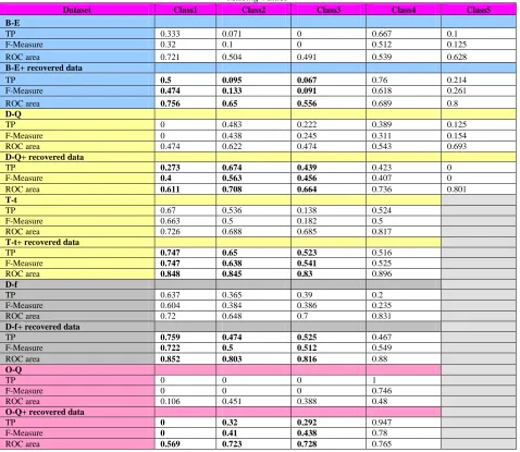
In this experiment as our previous work we want to show the effect of this algorithm on each class as well. The results are shown in Table3 and Table4. These tables show the evaluation measures of TP, F-Measure and ROC area after classification process. In Table3 top section shows the evaluation measures for original datasets with rows with missing values removed after training Meta learner and bottom section shows the same process on the datasets with recovered data using LS method.
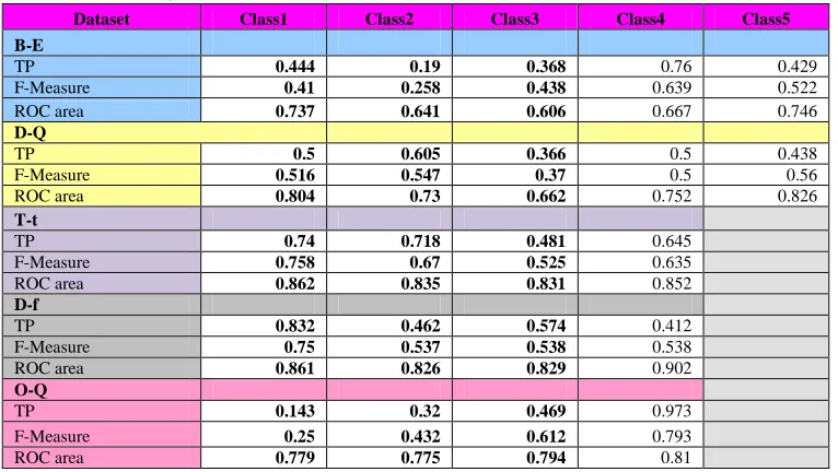
In Table4 we show the results of the modeling data after application of DCBA algorithm.
ISSN: 1992-8645 www.jatit.org E-ISSN: 1817-3195 5.CONCLUSIONS
This paper has presented The Mixture Model (TMM) combining the LS method and DCBA algorithm. The method has been proposed for the situations when there are considerable proportion of rows with missing values and when there are highly correlated features.
The results on fives dataset are very promising. The method can be effectively used in the cases when the data need to be complete and when the better performance is needed for further data analysis.
In the future we want to concentrate on analyzing the data using other statistical measures and also examine the effectiveness of the method on datasets with different characteristics.
REFERENCES:
[1] G. k. Bhattacharyya. and R. A. Johnson. “Statistical Concepts and Methods”. 1977, John Wiley and Sons.
[2] L. Malazizi, D. Neagu and Q. Chaudhry, “Improving Imbalanced Multidimensional Dataset Learner Performance with Artificial Data Generation: Density based Class-Boost Algorithm”, Proceeding of Industrial Conference on Data Mining (ICDM),
Germany, 2008, pp. 165-176, ISBN 978-3-540-70717-2.
[3] I. Wasitoand B. Mirkin, “Nearest neighbours in least-squares data imputation algorithms with different missing patterns”,
Computational Statistics and Data Analysis,
Vol. 50, No. 4, 2006, pp. 926-949.
[4] T. Hastie, R. Tibshirani, G. Sherlock, M. Eisen, P. Brown and D. Boststein, “Imputing missing data for gene expression arrays”,
Technical Report, Division of Biostatistics,
Stanford University, 1999.
[5] O. Troyanskaya, M. Cantor, G. Sherlock, P. Brown, T. Hastie, R. Tibshirani, D. Botstein and R.B. Altman, ”Missing value estimation methods for DNA microarrays”,
Bioinformatics, Vol. 17, 2001, pp. 520-525.
[6] S. Laaksonen, “Regression-based nearest neighbour hot decking”, Computational Statistics, Vol. 15, 2000, pp. 65-71.
[7] R.J.A. Little and D.B. Rubin, “Statistical analysis with missing data”, John Wiley and Sons, New York, 1987.
[8] R. R. Quinlan, “Unknown attribute values in induction”, Sixth International Machine Learning Workshop, NewYork, 1989.
[9] R. Pearson, “The Problem of Disguised Missing Data”. SIGKDD Exploration, . Vol. 8, No. 1, pp. 83-92.
[10] Y. Yuan, “Multiple Imputation for Missing Data: Concepts and New Development”. SAS Institute Inc, Rockville.
[11] M. A. Maloof, “Learning When Data Sets are Imbalanced and When Costs are Unequal and Unknown”. ICML Workshop on Learning from
Imbalanced data sets II, 2003.
[12] S. Ertekin, J. Huang, L. Bottou, C. L. Giles.” Learning on the Border: Active Learning In Imbalanced Data Classiffication”. CIKM07, Lisbon, Portugal, 2007.
[13] I. H. Witten and E. Frank, “Data Mining Practical Machine Learning Tools and Techniques with Java Implementation”. Morgan Kaufmann, 2000.
ISSN: 1992-8645 www.jatit.org E-ISSN: 1817-3195
Table 2: Classification Accuracy By 10-Fold Cross Validation,; Data With Missing Values Removed(Data1), Data1 Modeled Using DBCA Algorithm, Data With Empty Rows Recovered(Data2) And Data2 Modeled With TMM Algorithm
Datasets Cross-Validation: Overall Accuracy (%)
B-E D-Q T-t D-f O-Q
data1 with empty rows removed 35.443 31.4607 54.1667 47.549 58.1395
data1 modeled using DCBA algorithm 45.45 41 57 49 56.3
data2 with empty rows recovered 44.9153 45.8647 66.358 61.1111 66.6667
data2 modeled using TMM algorithm 51.6393 48.5915 68.2635 64.1935 69.7842
Table 3: Shows TP, F-Measure And ROC Area Statistics For All Classes In Five Datasets Before And After Recovering Missing Values
Dataset Class1 Class2 Class3 Class4 Class5
B-E
TP 0.333 0.071 0 0.667 0.1
F-Measure 0.32 0.1 0 0.512 0.125
ROC area 0.721 0.504 0.491 0.539 0.628
B-E+ recovered data
TP 0.5 0.095 0.067 0.76 0.214
F-Measure 0.474 0.133 0.091 0.618 0.261
ROC area 0.756 0.65 0.556 0.689 0.8
D-Q
TP 0 0.483 0.222 0.389 0.125
F-Measure 0 0.438 0.245 0.311 0.154
ROC area 0.474 0.622 0.474 0.543 0.693
D-Q+ recovered data
TP 0.273 0.674 0.439 0.423 0
F-Measure 0.4 0.563 0.456 0.407 0
ROC area 0.611 0.708 0.664 0.736 0.801
T-t
TP 0.67 0.536 0.138 0.524
F-Measure 0.663 0.5 0.182 0.5
ROC area 0.726 0.688 0.685 0.817
T-t+ recovered data
TP 0.747 0.65 0.523 0.516
F-Measure 0.747 0.638 0.541 0.525
ROC area 0.848 0.845 0.83 0.896
D-f
TP 0.637 0.365 0.39 0.2
F-Measure 0.604 0.384 0.386 0.235
ROC area 0.72 0.648 0.7 0.831
D-f+ recovered data
TP 0.759 0.474 0.525 0.467
F-Measure 0.722 0.5 0.512 0.549
ROC area 0.852 0.803 0.816 0.88
O-Q
TP 0 0 0 1
F-Measure 0 0 0 0.746
ROC area 0.106 0.451 0.388 0.48
O-Q+ recovered data
TP 0 0.32 0.292 0.947
F-Measure 0 0.41 0.438 0.78
[image:5.612.69.547.222.637.2]ISSN: 1992-8645 www.jatit.org E-ISSN: 1817-3195
Table 4: Shows TP, F-Measure And Roc Area Statistics For All Classes In Five Datasets With TMM
Dataset Class1 Class2 Class3 Class4 Class5
B-E
TP 0.444 0.19 0.368 0.76 0.429
F-Measure 0.41 0.258 0.438 0.639 0.522
ROC area 0.737 0.641 0.606 0.667 0.746
D-Q
TP 0.5 0.605 0.366 0.5 0.438
F-Measure 0.516 0.547 0.37 0.5 0.56
ROC area 0.804 0.73 0.662 0.752 0.826
T-t
TP 0.74 0.718 0.481 0.645
F-Measure 0.758 0.67 0.525 0.635
ROC area 0.862 0.835 0.831 0.852
D-f
TP 0.832 0.462 0.574 0.412
F-Measure 0.75 0.537 0.538 0.538
ROC area 0.861 0.826 0.829 0.902
O-Q
TP 0.143 0.32 0.469 0.973
F-Measure 0.25 0.432 0.612 0.793