Identifying Real Estate Opportunities using Machine
Learning
Alejandro Baldominos1,2* , Antonio José Moreno2, Rubén Iturrarte2, Óscar Bernárdez2and Carlos Afonso2
1 Computer Science Department, Universidad Carlos III de Madrid, Leganés, Spain 2 Artificial Intelligence Group, Rentier Token, Madrid, Spain
* Correspondence: [email protected]; Tel.: +34-91-624-6258
Version October 15, 2018 submitted to Preprints
Abstract: The real estate market is exposed to many fluctuations in prices, because of existing 1
correlations with many variables, some of which cannot be controlled or might even be unknown. 2
Housing prices can increase rapidly (or in some cases, also drop very fast), yet the numerous listings 3
available online where houses are sold or rented are not likely to be updated that often. In some cases, 4
individuals interested in selling a house (or apartment) might include it in some online listing, and 5
forget about updating the price. In other cases, some individuals might be interested in deliberately 6
setting a price below the market price in order to sell the home faster, for various reasons. In this 7
paper we aim at developing a machine learning application that identifies opportunities in the real 8
estate market in real time, i.e., houses that are listed with a price substantially below the market price. 9
This program can be useful for investors interested in the housing market. We have focused in a use 10
case considering real estate assets located in the Salamanca district in Madrid (Spain) and listed in the 11
most relevant Spanish online site for home sales and rentals. The application is formally implemented 12
as a regression problem, that tries to estimate the market price of a house given features retrieved 13
from public online listings. For building this application, we have performed a feature engineering 14
stage in order to discover relevant features that allows attaining a high predictive performance. 15
Several machine learning algorithms have been tested, including regression trees,k-nearest neighbors, 16
support vector machines and neural networks, identifying advantages and handicaps of each of 17
them. 18
Keywords:real estate; appraisal; investment; machine learning; artificial intelligence 19
1. Introduction 20
The real estate market is rapidly evolving. A recent report published by MSCI estimates the size 21
of the professionally managed real estate investment market in $8.5 trillion in 2017, increasing a total 22
of $1.1 trillion since the previous year [1]. Of course, the real market size is expected to be much larger 23
when counting assets which are not professionally managed or that are not object of investment. 24
When looked from a macroeconomic perspective, there are many aspects that significantly drive 25
the behavior of this market, such as demographics, interest rates, government regulation and, for short, 26
global economic health. 27
However, looking at the market evolution from a global perspective turns out to be too simplistic. 28
Although the market at a global scale is very tightly correlated, there are many aspects influencing the 29
behavior of markets at a local scale, such as political instability or the emergence of highly demanded 30
“hot spots" that can shift rapidly. Also, different market segments evolve at different paces, such as 31
high-end luxury condos. 32
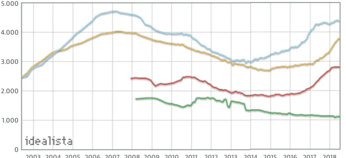
An example of such differences can be observed in Figure1, which shows the evolution of the 33
price (measured in euros per square meter) of resale houses in four different Spanish regions: Barcelona 34
(blue), Madrid (yellow), Palma de Mallorca (red) and Lugo (green). Data for Barcelona and Madrid are 35
available since 2002, whereas for Palma de Mallorca and Lugo are available after 2008. 36
2 of 20
Figure 1. Evolution of the Spanish resale real estate market, focusing on four different regions: Barcelona (blue), Madrid (yellow), Palma de Mallorca (red) and Lugo (green). Source: Idealista [2].
Attending to the figure we can see some common patterns in the evolution of Barcelona’s and 37
Madrid’s markets, which are the two largest metropolitan areas in Spain: a growth in the early 2000s 38
with a maximum in 2007, followed by a fall after 2008 due to the global financial crisis, which lasted 39
until 2015, a moment after which prices have started to recover almost reaching maximum values 40
again as of 2018. 41
Meanwhile, in Palma de Mallorca, which is a remarkable vacational place, the increase in the last 42
two years is more pronounced than in Madrid and Barcelona. On the other hand, in Lugo, which is 43
occupied mostly by rural areas, prices increased slightly in 2011, but are steadily decreasing since then. 44
The figure clearly shows how although some global patterns can be found in the evolution, each region 45
still shows some specificities in the prices evolution. 46
Of course, higher variability can be found when looking at specific assets. Most important factors 47
driving the value of a house are the size and the location, but there are many other variables that are 48
often taken into account when determining its value: number of bedrooms, proximity to some form 49
of public transport (buses, underground, etc.), number and quality of schools in the area, shopping 50
opportunities, availability of an elevator (in apartments located in higher floors), availability of gardens 51
or parks, etc. But certainly, the main reason ultimately determining the value of houses is demand. 52
With such a high variability and unpredictable factors (e.g., one neighborhood deemed better or 53
more fashionable than others) it is likely that the price of some assets will deviate from its expected 54
value. When the actual price is much less than the expected value, we could be dealing with an 55
investment opportunity: an asset that could generate immediate profit if sold soon after its purchase. 56
There can be a number of reasons motivating the existence of these investment opportunities, from 57
which two can be easily identified. The first one can occur when the seller publishes the advertisement 58
in some online listing. In that case, it could occur that the seller ignored the actual value of the house. 59
More likely, the house has remained published in the listing for some time, during which its value has 60
risen (because of global or local trends) but the seller has not updated its value. In the second case, the 61
asset price can be deliberately set lower than its expected value with the intention of it be sold fast, for 62
example if the seller needs the money. 63
Whichever the case, investment opportunities in real estate exist and can be identified. In this 64
paper, we aim at using machine learning techniques to identify such opportunities, by determining 65
whether the price of an asset is smaller than its estimated value. In particular, we have considered a 66
dataset of real estate assets located in the Salamanca district of Madrid, Spain, and listed in Idealista, 67
the most relevant Spanish online site for home sales and rentals, during the second semester of 2017. 68
The remainder of this paper is structured as follows: Section2describes the state of the art in 69
prediction of houses prices, and places this work in its context. Later, section3describes the dataset 70
Preprints (www.preprints.org) | NOT PEER-REVIEWED | Posted: 15 October 2018 doi:10.20944/preprints201810.0297.v1
used to train the models, with the machine learning techniques being described in section4. An 71
evaluation of the system is performed and its setup and results are discussed in section5. Finally, some 72
conclusive remarks and future lines of work are provided in section6. 73
2. State of the Art 74
Traditional models used for the appraisal or estimation of real estate assets have relied in hedonic 75
regression, which breaks the asset apart into its constituent characteristics in order to establish a 76
relationship between each of these and the price of the property. The model learned with hedonic 77
regression can then be used to estimate the price of an asset whose characteristics are known in advance. 78
In recent years, two works using this method have been presented by Jiang et al. [3,4] focusing on 79
properties in Singapore with sale transactions between 1995 and 2014. The data used by the authors 80
comprise a total of 315,000 transactions related to 216,000 dwellings in 4,820 buildings, from which 81
some were resales. Properties considered by authors to generate the model are the location, specified 82
as the postal district, the property type (apartment or condominium) and the ownership type (99 years, 83
999 years or freehold). 84
Some related work is concerned with trying to estimate the health of a real estate market using 85
data obtained from search queries and news. In these cases, the housing index price (HPI) is often used 86
as a proxy to determine the status of such market. As an example, Greenstein et al. [5] hypothesized 87
that search indices are correlated with the underlying conditions of the US housing market, and relied 88
on search data obtained from Google Trends as well as housing market indicators for testing that 89
hypothesis. It is remarkable that authors state that traditional forecasting had often relied on statistics 90
provided in annual reports, financial statements, government data, etc., which are often published 91
with significant delay and do not provide enough data resolution. To validate their hypothesis, a 92
seasonal autoregressive model was used to estimate the relationship. In the end, they are capable 93
of predicting home sales using online search, and also the house price index and demand for home 94
appliances. However, this does not allow the prediction of individual real estate assets. A similar 95
work was also published the same year by Sun et al. [6] who base their research on the fact that 90% 96
buyers and 92% sellers rely on the Internet for finding or posting information about properties. In their 97
work, authors propose combining online daily news sentiments with search engine data from Baidu 98
for predicting the house price index. Prediction models are trained using support vector regression, 99
artificial neural networks trained with back-propagation and radial basis functions neural networks, 100
and tested on data retrieved from Beijing, Shanghai, Chengdu and Hangzhou. 101
Other works rely on expert systems based on fuzzy logic, because of the similarity between 102
this technique and the human approach to decision making [7]. For example, Guan et al. [8] have 103
used adaptive neuro-fuzzy inference system (ANFIS) for real estate appraisal. To do so, they have 104
used data from 20,192 sales records in a mid-western city of the US between 2003 and 2007, which 105
were finally reduced to 16,523 after manual curation. The features comprised by this data include 106
location, year of construction and sale, square footage in each floor (including basement and garage), 107
number of baths, number of fireplaces, presence of central air, lot type, construction type, wall type and 108
basement type. Their approach combines neural networks with fuzzy inference, and authors report 109
mean average percentage errors for different age bands and different variables sets. It can be seen that 110
ANFIS outperform multiple regression analysis (MRA), although in some cases using location only 111
instead of all variables can improve results. In 2016, Sarip et al. [9] presented a work where they used 112
fuzzy least-squares regression FLSR to build a model from 352 properties in the district of Petaling, 113
Kuala Lumpur. For constructing the model, eight variables were considered: land area, built-up area, 114
number of bedrooms, number of bathrooms, building age, repair condition, quality of furniture and 115
location, along with the price in Malaysian ringgits (MYR). Those features which were categorial were 116
first converted into numeric attributes to be manageable by the model. Authors reported a mean 117
absolute error around 183,000 for FLSR, smaller than ANFIS and artificial neural networks. Finally, 118
4 of 20
situations of a real estate market with imprecise information, showing a case study which focused in 120
the purchase of one office building. Interestingly, del Giudice et al. state that while there is a wide 121
theoretical background regarding real estate investment, empirical support for such theory is scarce in 122
the literature. 123
A work by Rafiei et al. [11] presents an innovative approach where the focus is placed not in 124
property appraisal but in decision making at the time of starting a new construction, i.e., whether “to 125
build or not to build", in the words of the authors. Authors describe the use of a deep belief restricted 126
Boltzmann machine for learning a model from 350 condos (3-9 stories) built in Tehran (Iran) between 127
1993 and 2008. From these condos, a total of 26 attributes are used to train the model. Seven attributes 128
refer to physical and financial properties of the constructions, such as the ZIP code, the total floor 129
area and the lot area, the estimated construction cost per square meter, the duration of construction 130
and the price of the unit at the beginning of the project. Authors also retrieved additional economic 131
variables, which included regulation in the area, prices index, financial status in the construction area, 132
currency exchange rate, population and demographics, etc. When evaluating their model over a test 133
set of another 10 condos they obtain a test error as low as 3.6%, a number better than that attained 134
using neural networks trained with backpropagation. 135
Finally, some authors have relied on the use of machine learning techniques for estimating 136
or predicting the price of individual real estate assets. It is the case of Park and Kwon Bae [12], 137
who have analyzed housing data of 5,359 townhouses in Fairfax County, Virginia, combined from 138
various databases, from 2004 and 2007. These assets had 76 attributes, from which 28 were eventually 139
selected after filtering using at-test and logistic regression. Sixteen of these features are physical 140
features, referring to the number of bedrooms and bathrooms, number of fireplaces, total area, cooling 141
and heating systems, parking type, etc. Besides, three variables refer to the ratings of elementary, 142
middle and high schools in the area, and other eight refer to the mortgage contract rate, location and 143
construction and sale date. The last attribute is the class, which the authors have converted in binary: 144
either the closing price is larger than the listing price or the other way around. Therefore, the problem 145
can be seen as a classification to decide whether an investment is worthy or not instead of a regression 146
problem. For performing classification, authors compare different algorithms: decision trees (C4.5), 147
RIPPER, Naive Bayes and AdaBoost. Best results are achieved using RIPPER (repeated incremental 148
pruning to produce error reduction), a propositional rule learner, with an average error of about 25%. 149
Authors do not provide more specific metrics such as F1 score which allows to determine the model 150
goodness regardless of the class distribution. 151
Another work was presented by Manganelli et al. [13] in 2016, where the focus is put on appraisal 152
based on 148 sales of residencial property in a city of the Campania region, Italy. Considered variables 153
are the age of the property, date of sale, internal area, balconies area, connected area, number of 154
services, number of views, maintenance status and floor level. Authors used linear programming to 155
analyze the real estate data, learning the coefficients for the model, achieving an average percentage 156
error of 7.13%. 157
Finally, two more works have been published by del Giudice et al. [14,15] in 2017. In the first of 158
these works, authors use a genetic algorithm (GA) to try to establish a relationship between rental 159
prices and the location of assets in a central urban of Naples divided into five subareas, considering 160
also the commercial area, maintenance status and floor to be relevant parameters. The way in which the 161
authors use the GA is towards learning weights for these parameters, effectively building a regression 162
model which could be used for estimating rental prices. The obtained absolute average percentage 163
error is equal to 10.62%. In the second work, authors rely on Markov chain hybrid Monte Carlo method 164
(MCHMCM), yet they also tested neural networks, MRA and penalized spline semiparametric method 165
(PSSM). The model is again used for predicting the price of real estate properties in the center of 166
Naples, with the dataset comprising only 65 housing sales in twelve months. Besides the variables 167
from the previous work, they also considered the number of bathrooms, outer surface, panoramic 168
Preprints (www.preprints.org) | NOT PEER-REVIEWED | Posted: 15 October 2018 doi:10.20944/preprints201810.0297.v1
quality, occupancy status and distance from the funicular station. The MCHMCM model achieves an 169
absolute average percentage error of 6.61%, a better rate that the tested alternatives. 170
As shown in this section, literature on the application of machine learning to the valuation of real 171
estate assets is relatively scarce, at least in the way we are approaching the problem. While the few last 172
works cited in this section adhere to the same approach than ours, those works are restricted to certain 173
areas and only probes a small set of techniques. In this work, we will also focus on the snapshot of the 174
real estate market in a small region during a period of six months, yet evaluating additional machine 175
learning techniques, and approaching the problem as a regression task. 176
3. Data 177
In this paper, we will be focusing in a small segment of the market, comprising high-end real 178
estate assets located in the Salamanca district in Madrid, Spain. The city of Madrid is the capital of 179
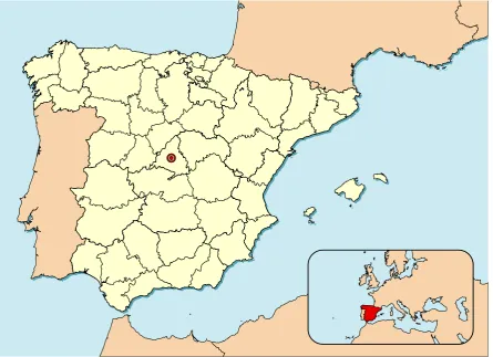
Spain and also the largest city, with more than 3 million residents. Its location within Spain (and also 180
framed within the context of the European continent) is shown in Figure2. The city is divided into 181
21 administrative divisions called districts. The Salamanca district is located to the north-east of the 182
historical center (see Figure3) and is home to 150,000 people, being one of the wealthiest and more 183
expensive places in Madrid and Spain. 184
3.1. Source and Description 185
In order to identify opportunities within the framework of a stable market, we have used data 186
from all residences costing more than one million euros, listed in Idealista (the more relevant Spanish 187
online platform for real estate sales and rentals) in the second semester of 2017 (from June 1st to 188
December 31st). 189
6 of 20
Figure 3.Location of the Salamanca district within the city of Madrid.
The raw data used for training the machine learning models comprise several attributes, which 190
can be grouped in three categories: location, home characteristics and ad characteristics. In particular, 191
the features involved in determining the location of the real estate asset are the following: 192
• Zone: division within the Salamanca district where the asset is located. This zone is determined 193
by Idealista based on the asset location. 194
• Postal code: the postal code for the area where the asset is located. 195
• Street name: the name of the street where the asset is located. 196
• Street number: number within the street where the asset is located. 197
• Floor number: the number of the floor where the asset is located. 198
The features defining the asset characteristics are the following: 199
• Type of asset: whether the asset is an apartment (flat, condo...) or a villa (detached or 200
semi-detached house). 201
• Constructed area: the total area of the asset indicated in square meters. 202
• Floor area: the floor area of the asset indicated in square meters, which will in some cases be 203
smaller than the constructed area, because terraces, gardens, etc. are ignored in this feature. 204
• Construction year: construction year of the building. 205
• Number of rooms: the total number of rooms in the asset. 206
• Number of baths: the total number of bathrooms in the asset. 207
• Is penthouse: whether the asset is a penthouse. 208
• Is duplex: whether the asset is a duplex, i.e., a house of two floors connected by stairs. 209
• Has lift: whether the building where the asset is located has a lift. 210
• Has box room: whether the asset includes a box room. 211
• Has swimming pool: whether the asset has a swimming pool (either private or in the building). 212
• Has garden: whether the asset has a garden. 213
• Has parking: whether the asset has a parking lot included in the price. 214
• Parking price: if a parking lot is offered by an additional cost, then that price is specified in this 215
feature. 216
• Community costs: the monthly fee for community costs. 217
Finally, the features defining the ad characteristics are the following: 218
• Date of activation: the date when the ad was published in the listing and displayed publicly. 219
Preprints (www.preprints.org) | NOT PEER-REVIEWED | Posted: 15 October 2018 doi:10.20944/preprints201810.0297.v1
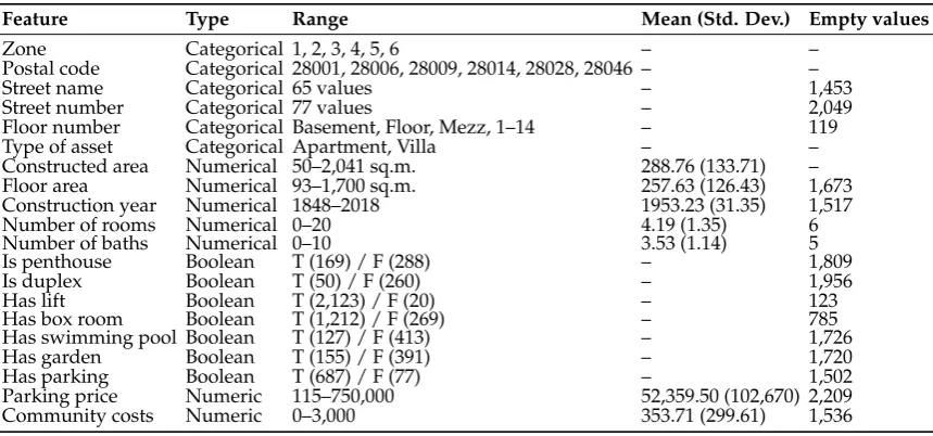
Table 1. Data description, showing the range of values for each feature and the number of empty values, as well as mean and standard deviation in the case of numerical values.
Feature Type Range Mean (Std. Dev.) Empty values
Zone Categorical 1, 2, 3, 4, 5, 6 – –
Postal code Categorical 28001, 28006, 28009, 28014, 28028, 28046 – –
Street name Categorical 65 values – 1,453
Street number Categorical 77 values – 2,049
Floor number Categorical Basement, Floor, Mezz, 1–14 – 119
Type of asset Categorical Apartment, Villa – –
Constructed area Numerical 50–2,041 sq.m. 288.76 (133.71) – Floor area Numerical 93–1,700 sq.m. 257.63 (126.43) 1,673 Construction year Numerical 1848–2018 1953.23 (31.35) 1,517
Number of rooms Numerical 0–20 4.19 (1.35) 6
Number of baths Numerical 0–10 3.53 (1.14) 5
Is penthouse Boolean T (169) / F (288) – 1,809
Is duplex Boolean T (50) / F (260) – 1,956
Has lift Boolean T (2,123) / F (20) – 123
Has box room Boolean T (1,212) / F (269) – 785
Has swimming pool Boolean T (127) / F (413) – 1,726
Has garden Boolean T (155) / F (391) – 1,720
Has parking Boolean T (687) / F (77) – 1,502
Parking price Numeric 115–750,000 52,359.50 (102,670) 2,209 Community costs Numeric 0–3,000 353.71 (299.61) 1,536
• Date of deactivation: the date when the ad was removed from the listing, which could indicate 220
that it was already sold or rented. 221
• Price: current price of the asset, or price when the ad was deactivated, which in most cases 222
corresponds to the price at which the asset was sold or rented. 223
Some of the previous features might not be available. This will happen in most cases because 224
the seller has not explicitly specified some information about the asset, for example, whether a lift 225
is available, which are the monthly community costs, etc. Regarding the street name and number, it 226
can be intentionally hidden by the seller, so potential buyers are not aware of the actual location of 227
the building. Some information is always available, such as the zone, postal code, constructed area, 228
number of rooms and number of bathrooms. 229
In the dataset, there is a total of 2,266 real estate assets, from which 2,174 are apartments and 92 230
are villas. The assets prices range between 1 and 90 million euros, with an average price of about 2.02 231
million and a median price of about 1.66 million. More information about the data and the range of 232
values is available in Table1. 233
3.2. Data Cleansing 234
Before starting to work with the data, we have proceeded to clean some of the data. Although the 235
data is relatively clean, some information is particularly noisy because the way it is communicated by 236
sellers in the listing. 237
An example is the street name, which is a free text field. For this reason, there was no consensus 238
regarding some aspects such as capitalization, prepositions or accents. We have manually revised this 239
field in order to standardize it according to the actual street names gathered in the streets guide. 240
The floor area is not specified in most of the cases. In this case, we have assumed it to be equal to 241
the constructed area. Even when this is a rough estimate, it is often the case than the floor area is only 242
slightly smaller than the constructed area, and therefore we have considered this estimation to be an 243
appropriate proxy. 244
Finally, for all binary features, we have considered empty values as non-availability of the 245
corresponding features. This seems reasonable within the scope of online listings, since it is more 246
likely that the seller fills the field when the feature is available. For example, in the case of swimming 247
8 of 20
Figure 4.Matrix of correlations between each pair of variables.
not include a swimming pool. We will consider that for those ads where no information is provided 249
about the pool (in this case, a total of 1,726), then such a pool is not available. 250
3.3. Exploratory Data Analysis 251
Before proceeding with the training of machine learning models, we are interested in getting some 252
insights about the data at hand. In particular, it would be interesting to know how different variables 253
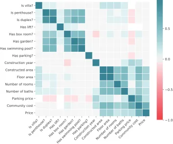
affect the price of the real estate model, to understand their potential quality as predictors. This 254
information is shown in Figure4, where the correlation between each pair of variables (considering 255
only binary and continuous variables) is shown. The Pearson correlation coefficient is computed for 256
continuous variables, and the point biserial correlation coefficient is computed for binary variables. 257
From the correlation matrix we can see that the main variables affecting the asset price are those 258
related to the house size, mainly the constructed area. Of course, all these variables, such as the area, 259
number of bedrooms and number of bathrooms, are highly correlated among them. There is also a 260
significant impact of the monthly community cost, but in this case it is likely that the causality points 261
in the other direction: the cost grows for those houses which are more expensive. Interestingly, most of 262
the binary features as well as the construction year do not seem to have either positive or negative 263
correlation with the price. 264
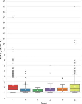
Figure5shows the distribution of asset prices based on their location, more specifically, based on 265
their zone attribute provided by Idealista. Although differences are not very noticeable, it can be seen 266
how assets in zone 1 have a substantially larger mean and median price when compared to the other 267
zones. Zones 2 and 3 have slightly lower prices than the rest of the zones. 268
To understand whether these variations can be explained because of the zone and not because of 269
other factors, we have also plotted the distribution of constructed areas per each zone, which can be 270
seen in Figure6. In this figure we can see how there are not remarkable differences between different 271
zones, with the exception of zone 4 where the median area is noticeably larger. When comparing the 272
Preprints (www.preprints.org) | NOT PEER-REVIEWED | Posted: 15 October 2018 doi:10.20944/preprints201810.0297.v1
Figure 5.Boxplot of the distribution of prices based on the asset location.
distributions of areas with the distribution of prices, we can conclude that the asset location is also a 273
factor when determining the price, beyond the constructed area itself. For example, it seems that zone 274
1 is more expensive in average, since prices are larger while areas follow a similar distribution than in 275
other areas. The opposite happens with zone 4, where prices are roughly the same but constructed 276
areas are larger. 277
Finally, we are interested in checking how a linear regression model can fit the prices based only 278
on the constructed area. We plot the regression model on Figure7, where two models are actually 279
plotted, one per each type of asset. Assets with prices larger than 8 million have been removed from 280
the figure to ease readability, since these assets are a minority. We can see how only the constructed 281
area is insufficient to accurately fit the prices, and therefore a more complex model involving more 282
predictions must be built for achieving successful prediction. 283
4. Machine Learning Proposal 284
In the previous section, we have seen how different variables correlate with the asset price, with 285
the constructed area being the attribute with a larger influence on the price. We have also graphically 286
seen how a linear regression model considering only the constructed area is insufficient for successfully 287
predicting the price. 288
In this work, we will use machine learning to build and train more complex models for carrying 289
out price prediction. This problem will be tackled as a multi-variate regression problem, with the price 290
being the output, where features can be binary (such as whether there is a swimming pool or a lift), 291
categorical (such as the asset location) or continuous (such as the constructed area). To be able to use 292
10 of 20
Figure 6.Boxplot of the distribution of constructed areas based on the asset location.
Figure 7.Linear regression between the constructed area and the asset price, based on the asset type.
This means that any categorical feature withNvalues will be transformed into a total ofNbinary 294
features. 295
Also, we know that the values for some of the features remain unknown in some instances. This 296
happens with the street name, the street number, the construction year, the parking price and the 297
community costs. Since the first feature is categorical, the problem of null values is resolved after 298
performing one-hot encoding (since all binary features can take the value “false"). As for the other 299
variables, we have decided to remove them from the data. This is especially important for the street 300
number, since it is not a relevant feature but could lead to overfitting (in some cases, the street name 301
and number identifies an asset). 302
Preprints (www.preprints.org) | NOT PEER-REVIEWED | Posted: 15 October 2018 doi:10.20944/preprints201810.0297.v1
Bearing in mind with these constraints, we have finally considered the use of four different 303
machine learning techniques: 304
• Support vector regression: this method is also known as a “kernel method”, and constitutes 305
an extension of classical support vector machine classifiers to support regression [16]. Kernel 306
methods transform data into a higher dimensional state where data can be separable by a 307
certain function, then learning such function to discriminate between instances. When applied to 308
regression, a parameter epsilon (e) is introduced, thus aiming that the learned function does not 309
deviate from the real output by a value larger than epsilon for each instance. 310
• k-nearest neighbors: this is an example of a geometric technique to perform regression. In this 311
technique, data is not really used to build a model, but is rather considered a “lazy” algorithm, 312
since it needs to traverse the whole learning set in order to carry out prediction for a single 313
instance. In particular, whatk-nearest neighbors does is compute the distance of the instance to 314
be predicted to all of the instances in the learning dataset, based on some distance function or 315
metric (such as Euclidean or cosine distance). Once distances are computed, thekinstances in 316
the training set which are closest to the instance subject of prediction will be retrieved, and their 317
known output will be aggregated to generate a predicted output, for example, by computing 318
their average. This method is interesting since it will consider assets similar to the one we want to 319
predict, but can be problematic when dealing with high-dimensional data with binary attributes. 320
• Ensembles of regression trees: regression trees are logical models that are able to learn a set of 321
rules in order to compute the output of an instance given its features. A regression tree can be 322
learned from a training dataset by choosing the most informative feature according to some 323
criterion (such as entropy or statistical dispersion) and then dividing the dataset based on some 324
condition over that feature. The process is repeated with each of the divided training subsets 325
until a tree is completely formed, either because no more features are available to be selected or 326
because fitting a regression model on the subset performs better than computing a regression 327
sub-tree. In this paper we will use ensembles of trees, which means that several models will be 328
combined in order to reduce regression bias. To build the ensemble, we will use the technique 329
known as extremely randomized trees, introduced by Geurts et al. [17] as an improvement to 330
random forests. 331
• Multi-layer perceptron: the multi-layer perceptron is an example of a connectionist model, more 332
particularly an implementation of an artificial neural networks. This kind of models comprise an 333
input layer that receives as input the values for the features of each instance and several hidden 334
layers, each of which features several hidden units, or neurons. The model is fully connected, 335
meaning that each neuron from one layer is connected to every single neuron in the following 336
layer. Each connection has a corresponding floating number, called weight, which serves for 337
aggregating the inputs to the neuron, and then a non-linear activation function is applied. During 338
training, a gradient descent algorithm is used to fit the connections weights via a process known 339
as backpropagation. 340
These algorithms can be configured based on different parameters, which can have an impact on 341
performance. In the following section, we describe the experimental setup along with the different 342
instantiations of parameters for testing each of the previously listed machine learning algorithms. 343
5. Evaluation 344
In this section, we will first introduce the experimental setup which has been applied for testing 345
different machine learning regression models. Then, we will describe the results and discuss relevant 346
findings. 347
5.1. Experimental Setup 348
As described in the previous section, we will test the performance of four different machine 349
12 of 20
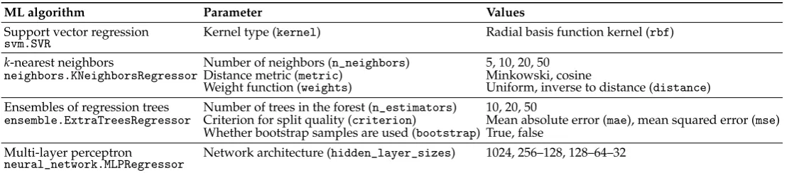
Table 2.Configuration in scikit-learn of the different machine learning algorithms that will be used for addressing the regression problem.
ML algorithm Parameter Values
Support vector regression Kernel type (kernel) Radial basis function kernel (rbf)
svm.SVR
k-nearest neighbors Number of neighbors (n_neighbors) 5, 10, 20, 50
neighbors.KNeighborsRegressorDistance metric (metric) Minkowski, cosine
Weight function (weights) Uniform, inverse to distance (distance) Ensembles of regression trees Number of trees in the forest (n_estimators) 10, 20, 50
ensemble.ExtraTreesRegressor Criterion for split quality (criterion) Mean absolute error (mae), mean squared error (mse) Whether bootstrap samples are used (bootstrap) True, false
Multi-layer perceptron Network architecture (hidden_layer_sizes) 1024, 256–128, 128–64–32
neural_network.MLPRegressor
of them can be configured according to different parameters. In this paper, we have considered the 351
following: 352
• Support vector regression: we will specify the kernel type. 353
• k-nearest neighbors: we will configure the number of neighbors to consider, the distance metric 354
and the weight function used for prediction. 355
• Ensembles of regression trees: we will set up the number of trees that conform the forest, the 356
criterion for determining the quality of a split and whether or not bootstrap samples are used 357
when building trees. 358
• Multi-layer perceptron: we will consider different architectures, i.e., different configurations of 359
how hidden units are distributed among layers. 360
For training machine learning models, we will use the scikit-learn package for Python [18], in its 361
version 0.19.2 (the latest as of August 2018). Table2describes the different configurations considered 362
for training the machine learning models. Also, the canonical names of the classes and the attributes 363
in the scikit-learn package are shown to ease reproducibility of the experiments. In the case of the 364
multi-layer perceptron, each number indicates the number of neurons in one layer, therefore the 365
configuration “256–128” means 256 units in the first hidden layer and 128 units in the second hidden 366
layer. 367
Additionally, some machine learning techniques perform better when data is normalized. In this 368
case, we will test out all techniques both with data normalized in the range [0, 1] and not normalized. 369
In order to normalize data, we have divided continuous features by the maximum value in the training 370
set. Of course, it could happen that some values in the test are larger than one, but that will not 371
constitute an issue. Normalizing data is important for some techniques to work properly: it is the case 372
of neural networks, where big values can lead to the vanishing or exploding gradient problem. 373
From the four techniques described before, two of them have an stochastic behavior: it is the case 374
of the ensembles of regression trees (where trees in the forest are built based on some random factors) 375
and of the multi-layer perceptron, where weights are initialized randomly. In order to reduce bias and 376
obtain significant results, we have run each of the experiments involving these techniques a total of 30 377
times. 378
Finally, in order to prevent biased results when sampling the dataset in order to build the train 379
and test sets, we will use 5-folds cross validation. In this approach, the whole dataset is first randomly 380
shuffled and then splitted into five equally sized folds. Five experiments will then be carried out: one 381
for each different fold used as the test set. The training set will always be made out of the remaining 382
four folds. When reporting results in the following section, all metrics will refer to the average of the 383
cross validation, i.e., will be computed as the average of the five results obtained for each of the test 384
sets (macro-average). 385
Preprints (www.preprints.org) | NOT PEER-REVIEWED | Posted: 15 October 2018 doi:10.20944/preprints201810.0297.v1
The total number of experiments that will be carried out is equal to 10 for the support vector 386
regression, 160 for thek-nearest neighbors, 3,600 for the ensembles of regression trees and 900 for the 387
multi-layer perceptron. It is worth noting that in all techniques, every combination of setups is run ten 388
times: once per fold both with normalized and not normalized data. In the latter two techniques, each 389
of these experiments is run 30 times. Therefore, the total number of experiments is 4,670. 390
5.2. Results and Findings 391
In this section, we will explore the performance achieved by different machine learning models. 392
The following quality metrics for regression have been computed, which are provided by the 393
scikit-learn API: 394
• Explained variance regression score, which measures the extent to which a model accounts for the variation of a dataset. Letting ˆybe the predicted output andythe actual output, this metric is computed as follows:
Evar(y, ˆy) =1−Var{y−yˆ}
Var{y}
In this equation,Varis the variance of a distribution. The best possible score is 1.0, which would 395
occur wheny=yˆ. 396
• Mean absolute error, which computes the average of the error for all the instances, computed as follows:
MAE(y, ˆy) = 1
n n
∑
i=0|yi−yˆi|
Since this is an error metric, the best possible value is 0. 397
• Median absolute error, similar to the previous score but computing the median of the distribution of differences between the expected and actual values:
MedAE(y, ˆy) =median(|y1−yˆ1|, . . . ,|yn−ynˆ |)
Again, since this is an error metric, the best possible value is 0. 398
• Mean squared error, similar to MAE but with all errors squared, and therefore computed as follows:
MSE(y, ˆy) = 1
n n
∑
i=0|yi−yˆi|2
As it happened with MAE, since this is an error metric, the best possible value is 0. 399
• Coefficient of determination (R2), which provides a measure of how well future samples are likely to be predicted. It is computed using the following equation:
R2(y, ˆy) =1−∑
n
i=0(yi−yˆi)2 ∑n
i=0(yi−y¯)2
In the previous equation, ¯yrefers to the average of the real outputs. The maximum value for 400
the coefficient of determination is 1.0, which would be obtained when the predicted output 401
matches the real output for all instances.R2would be 0 if the model always predicts the average 402
output, but it can also hold negative values, since the model can work arbitrarily worse than just 403
predicting the estimated value. 404
In order to discuss the results, we will address relevant findings which can be extracted from the 405
data. 406
Which model performs best? 407
When considering the mean absolute error for determining the best performers, we notice that 408
14 of 20
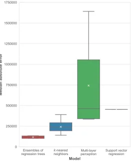
Figure 8.Boxplot of the distribution of median average errors per machine learning technique.
ten models are always ensembles, with either 10, 20 or 50 estimators. The split criterion, bootstrap 410
instances and normalization neither seem to have a significant effect on performance. The smallest 411
mean absolute error is 338,715 euros (a relative error of 16.80%). Consistent results are found when 412
considering the median absolute error, although best performers are not sorted on a side-by-side basis 413
(i.e., the model with the best MAE do not correspond to the model with the best MedAE). In this case, 414
all top-ten models are also ensembles of regression trees. The best median absolute error is 94,850 415
euros (a relative error of 5.71%). 416
The distribution of best median average errors per machine learning technique is shown in Figure 417
8. In this figure, we can see how ensembles of regression trees significantly outperform all of the 418
other techniques, followed byk-nearest neighbors, support vector regression and the multi-layer 419
perceptron. In the case of support vector regression, only one configuration was tested and the model 420
is deterministic, for this reason there is a single result instead of a distribution. As for the multi-layer 421
perceptron, a very large variance can be seen in the distribution of results, along with a remarkable 422
difference between the average and the median MedAE. Worst MAE and MedAE are always reported 423
by the multilayer-perceptron with a single layer with 1024 units. Because of the relatively small 424
availability of data, this model could be affected by overfitting, although further testing is required to 425
confirm this diagnosis. 426
Regarding the explained variance regression score and the coefficient of determination, both 427
metrics are highly correlated. The best model when assessed based onR2achieves a value of about 428
0.46 for both metrics. 429
How are models affected by setup? 430
The impact of parameters in the median absolute error for the different machine learning 431
techniques is shown in Figures 9, 10and 11 for the ensembles of regression trees, the k-nearest 432
neighbors and the multi-layer perceptron respectively. 433
Preprints (www.preprints.org) | NOT PEER-REVIEWED | Posted: 15 October 2018 doi:10.20944/preprints201810.0297.v1
Figure 9.Distribution of the median average error based on the different parameters for the ensembles of regression trees.
Figure 10.Distribution of the median average error based on the different parameters for thek-nearest neighbors.
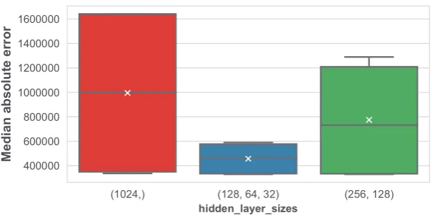
Figure 11.Distribution of the median average error based on the different parameters for the multi-layer perceptron.
As we can see, in the case of ensembles of regression trees the number of trees in the forest has 434
little impact in the performance. It seems that the mean MedAE slightly decreases as the number 435
of estimators grow, but the variation is very small. Variance also suffer a reduction as a result of 436
introducing more trees, although again this effect is barely perceptible. In the case of the use of 437
bootstrap sampling, it seems clear that its use negatively affects the model performance in a significant 438
manner. As for the split criterion, a slight reduction in MedAE follows the use of the median squared 439
16 of 20
Figure 12.Distribution of the median average error based on the use of normalization for the different machine learning techniques.
When studying the number of neighbors, a clear pattern is shown where the error grows 441
proportionally to the number of considered neighbors. Also, the variance in MedAE grows as well. 442
This is indicating that considering more similar instances is not only increasing variability but also 443
adding confusion to the regression. From the obtained results, it is left as future work to test this 444
technique with a number of neighbors smaller than five (like one or two) to test whether the error 445
keeps descending. Considering the weights of the different features when computing the nearest 446
neighbors, it is clear that weights that are inversely proportional to the distance of the target instance 447
to the neighbors work better than uniform weights. And regarding the distance metric, Minkowski 448
has also reported significantly better results than a cosine distance. 449
Finally, in the case of the multi-layer perceptron, results show that performance is very sensitive 450
to the architecture. It is interesting to see that the minimum MedAE is constant between different 451
alternatives, but the mean and median MedAE is much smaller as more layers with less units each 452
are introduced. As a result, variance is also affected, and we check that the configuration using three 453
hidden layers with 128 units in the first one is the one reporting the best average MedAE. Nevertheless, 454
as we concluded earlier, errors are always much larger than those obtained using ensembles of 455
regression trees ork-nearest neighbors. 456
When does normalization provide an advantage? 457
The impact of the use of normalization in the median average error is shown in Figure12for the 458
different machine learning techniques considered in this paper. 459
From this figure, we can see how normalization does not have an impact in the ensembles of 460
regression trees,k-nearest neighbors and support vector regression. This occur due to the fact that 461
normalization results in a linear transformation of data. Therefore, in the case ofk-nearest neighbors, 462
the distance metric is consistent between any pair of instance after the linear transformation of their 463
features. The same thing happens when using support vector machines, and when using such features 464
for building a regression tree. 465
The only case in which normalization makes a difference is when using a multi-layer perceptron. 466
Interestingly, in this case the median average error increases when normalization is used. This is 467
contrary to the common belief, where normalization is often considered a good practice to prevent 468
numerical instability when training the neural network. In this paper, we will not study the causes 469
of this issue in further detail, since it has been proved that the perceptron is not competitive when 470
compared to other machine learning techniques in the problem of real estate price prediction. Therefore, 471
Preprints (www.preprints.org) | NOT PEER-REVIEWED | Posted: 15 October 2018 doi:10.20944/preprints201810.0297.v1
Table 3. Average (and standard deviation) of training and prediction times for different machine learning configurations.
ML algorithm Parameter Value Train time (s) Predict time (s) Support vector regression – – 0.500 (0.022) 0.093 (0.0015)
Ensembles of regression trees
n_estimators 1020 0.999 (1.068)2.037 (2.185) 0.0011 (0.00006)0.0021 (0.00011)
50 5.192 (5.587) 0.0049 (0.00024)
bootstrap true 1.752 (2.250) 0.0026 (0.0015)
false 3.734 (4.905) 0.0028 (0.0017)
criterion maemse 5.337 (4.195)0.149 (0.103) 0.0027 (0.0016)0.0027 (0.0016)
k-nearest neighbors
n_neighbors
5 0.0016 (0.0014) 0.013 (0.0038)
10 0.0017 (0.0015) 0.014 (0.0036)
20 0.0017 (0.0016) 0.015 (0.0031)
50 0.0016 (0.0015) 0.018 (0.0016)
weights distanceuniform 0.0017 (0.0015)0.0016 (0.0014) 0.015 (0.0035)0.015 (0.0037)
metric cosine 0.00027 (0.000012) 0.018 (0.0013)
minkowski 0.0030 (0.00038) 0.012 (0.0031)
Multi-layer perceptron hidden_layer_sizes (128, 64, 32)(256, 128) 1.727 (1.104)3.045 (1.487) 0.00076 (0.00013)0.0011 (0.000061)
(1024) 8.376 (0.094) 0.0021 (0.000061)
a more thorough study of the causes, involving how the loss value evolves with the training epochs is 472
left for future work. 473
How much time do models require to train and run?Training and exploitation times can be a critical 474
aspect of running a machine learning model in a production setting. For this reason, in this paper we 475
have decided to introduce a study of how times vary depending on the machine learning technique 476
and its specific setup. It is worth recalling that times reported in this section refer to training and 477
testing within cross-validation setting, where training is done with 80% of the instances (1,813 assets) 478
and testing with the remaining 20% (453 assets). 479
The average time, along with the standard deviation, for both training and prediction of the 480
different machine learning models and configurations is shown in Table3. In general, we can see how 481
k-nearest neighbors is a lazy ML algorithm, where the training time is negligible when compared with 482
the prediction time; whereas this effect does not happen in other techniques. 483
For such reason,k-nearest neighbors is the fastest algorithm to train, and no significant differences 484
are found for different setups, with the only exception of the distance metric. The reason of Minkowski 485
requiring more time than the cosine distance is that when Minkowski is used, some pre-processing can 486
be done during training in order to accelerate prediction (such as building a KD-tree or a Ball-tree). As 487
a result, training is faster when this pre-processing is not done (because it is not possible using a cosine 488
distance) but prediction is slower. 489
Support vector regression’s training is relatively fast when compared to the neural network 490
models or ensembles of trees, but prediction time is about two orders of magnitude higher. 491
In the case of ensembles, it can be seen how the setup has a remarkable effect on both training and 492
prediction time. These times scale linearly with the number of trees, which is an expected behavior. 493
The use of bootstrap instances and the split criterion do not affect the prediction time, but impact 494
significantly the cost of training. This cost is specially sensitive to the training split criterion, where 495
computing the MAE requires about 50 times the time of computing the MSE. This is likely to be due to 496
implementation details of the error computation. 497
Finally, in the case of the multi-layer perceptron, times are in a similar scale than those of the 498
ensembles. Interestingly, the time in this case decreases as more layers are added, given that the 499
number of units is smaller. This is likely to be due to the implementation, although a deeper study is 500
18 of 20
6. Conclusions and Future Work 502
The real estate market constitutes a good setting for investing, due to the many aspects governing 503
the prices of real estate assets and the variances that can be found when looking at local markets and 504
small-scale niches. 505
In this paper, we have explored the application of diverse machine learning techniques with the 506
objective of identifying real estate opportunities for investment. In particular, we have focused first in 507
the problem of predicting the price of a real estate asset whose features are known, and have modelled 508
it as a regression problem. 509
We have performed a thorough cleansing and exploration of the input data, after which we have 510
decided to build machine learning models using four different techniques: ensembles of regression 511
trees, k-nearest neighbors, support vector machines for regression and multi-layer perceptrons. 512
Cross-validation of five folds have been used in order to avoid biases resulting from the split in 513
train and test subsets. Because we understand that the parameterization of the different techniques 514
can drive significant variations in the performance, we have identified some of the potentially most 515
influencing parameters and tested different setups for those. We have also reported results on the use 516
of the algorithms after data normalization. 517
After training and evaluating the models, we have thoroughly studied the results, revealing 518
findings on how different setups impact the performance. Results prove that outperforming models 519
are always those consisting of ensembles of regression trees. In quantitative terms, we have found 520
that the smallest mean absolute error is 338,715 euros, and the best median absolute error is 94,850 521
euros. These errors can be considered high within the scope of financial investment, but are relatively 522
small under the fact that data comprise only assets with values over one million euros. In fact, when 523
the mean and median absolute errors are compared with the mean and median of the distribution of 524
prices, relative errors of 16.80% and 5.71% are obtained respectively. 525
In this sense, it is worth mentioning that the fact of the mean being much larger than the median 526
can be explained due to the presence of outliers. For example, the most expensive asset in the dataset 527
is priced 90 million dollars, and according to the description it is an apartment of 473 square meters 528
with five bedrooms and five bathrooms. This price seems to be excessive for an apartment of such 529
characteristics, meaning that either the price is a typo and the asset was sold at a much smaller price, 530
or the description has been recorded incorrectly. 531
In either case, further analysis of prediction errors, even involving manual assessment of experts, 532
is left for future work which can serve for improving the quality of the database and therefore of the 533
trained machine learning models. 534
Also, the evaluation of a model built usingk-nearest neighbors with a number of neighbors 535
smaller than five was left for future work. Additionally, further analysis on the impact of normalization 536
in the performance of the multi-layer perceptron can be of interest, since results reported in this paper 537
seems to contradict the common belief that normalization helps prevent numerical instability and can 538
ease faster convergence. Finally, the impact of different architectures in both regression error and time 539
are worth exploring. 540
Another field for potential research involves the use of deep learning techniques for extracting 541
relevant features from natural language descriptions. So far, these data have not been provided to 542
us, but all adverts have a description introduced by the seller describing the home at sale. A feature 543
vector extracted from this text, for example by using convolutional neural networks with temporal 544
components, could add a remarkable value to the features already known. 545
Finally, in this paper we have approached the problem of identifying investment opportunities as 546
a regression problem consisting on the estimation of the actual appraisal of the assets. However, if this 547
valuation were done manually, then the problem could be tackled as a binary classification problem, 548
where the objective would be to determine whether the asset itself is an investment opportunity; for 549
example, if the sale price were smaller than the valuation price. Exploring this research line is also 550
suggested as a future work. 551
Preprints (www.preprints.org) | NOT PEER-REVIEWED | Posted: 15 October 2018 doi:10.20944/preprints201810.0297.v1
Data Statement 552
This work has relied on data provided by Idealista, consisting on the list of real estate assets for 553
sale in the platform in the Salamanca district (Madrid, Spain) during the second semester of 2017 554
(between July 1st and December 31st, both inclusive). Due to our non-disclosure agreement with 555
Idealista, we are not allowed to publish or redistribute the dataset used for this work. For authors 556
aiming at reproducing experiments in this paper, we suggest contacting Idealista using the form 557
available in the following address:https://www.idealista.com/data/empresa/sobre-nosotros. 558
Conflicts of Interest 559
Some of the knowledge obtained from this paper or the machine learning models built in this 560
work might be implemented and/or commercialized in the future by Rentier, a company to which all 561
authors in the present work are affiliated. The authors declare no other conflicts of interest. 562
Acknowledgment 563
The authors would like to thank Beatriz Cámara and Alfonso Lozano from Idealista for their 564
collaboration in providing access to the data used in this paper and support. 565
References 566
1. Teuben, B.; Bothra, H. Real Estate Market Size 2017 – Annual Update on the Size of the Professionally 567
Managed Global Real Estate Investment Market. Technical report, MSCI, Inc., 2018. Available online: 568
https://www.msci.com/documents/10199/6fdca931-3405-1073-e7fa-1672aa66f4c2. 569
2. Idealista. Índice Idealista 50: Evolución del Precio de la Vivienda de Segunda Mano en España, 2018. 570
Available online:https://www.idealista.com/news/estadisticas/indicevivienda#precio. 571
3. Jiang, L.; Phillips, P.C.B.; Yu, J. A New Hedonic Regression for Real Estate Prices Applied to the Singapore 572
Residential Market. Technical report, Cowles Foundation Discussion Paper No. 1969, 2014. Available at 573
SSRN:https://ssrn.com/abstract=2533017. 574
4. Jiang, L.; Phillips, P.C.; Yu, J. New Methodology for Constructing Real Estate Price Indices Applied to the 575
Singapore Residential Market.Journal of Banking and Finance2015,61, S121–S131. 576
5. Greenstein, S.M.; Tucker, C.E.; Wu, L.; Brynjolfsson, E. The Future of Prediction : How Google Searches 577
Foreshadow Housing Prices and Sales The Future of Prediction How Google Searches Foreshadow Housing 578
Prices. InEconomic Analysis of the Digital Economy; The University of Chicago Press, 2015; pp. 89–118. 579
6. Sun, D.; Du, Y.; Xu, W.; Zuo, M.; Zhang, C.; Zhou, J. Combining Online News Articles and Web Search to 580
Predict the Fluctuation of Real Estate Market in Big Data Context. Pacific Asia Journal of the Association for 581
Information Systems2015,6, 19–37. 582
7. Zurada, J.; Levitan, A.; Juan, G. Non-Conventional Approaches to Property Vale Assessment. Journal of 583
Applied Business Research2016,22, 1–14. 584
8. Guan, J.; Shi, D.; Zurada, J.M.; Levitan, A.S. Analyzing Massive Data Sets: An Adaptive Fuzzy Neural 585
Approach for Prediction, with a Real Estate Illustration.Journal of Organizational Computing and Electronic 586
Commerce2014,24, 94–112. 587
9. Sarip, A.G.; Hafez, M.B.; Nasir Daud, M. Application of Fuzzy Regression Model for Real Estate Price 588
Prediction.Malaysian Journal of Computer Science2016,29, 15–27. 589
10. Del Giudice, V.; De Paola, P.; Cantisani, G. Valuation of Real Estate Investments through Fuzzy Logic. 590
Buildings2017,7, 26. 591
11. Rafiei, M.H.; Adeli, H. A Novel Machine Learning Model for Estimation of Sale Prices of Real Estate Units. 592
Journal of Construction Engineering and Management2016,142, 04015066. 593
12. Park, B.; Kwon Bae, J. Using Machine Learning Algorithms for Housing Price Prediction: The Case of 594
Fairfax County, Virginia Housing Data.Expert Systems with Applications2015,42, 2928–2934. 595
13. Manganelli, B.; Paola, P.D.; Giudice, V.D. Linear Programming in a Multi-Criteria Model for Real Estate 596
Appraisal. International Conference on Computational Science and its Applications, Part I, 2016, Vol. 9786, 597
20 of 20
14. Del Giudice, V.; De Paola, P.; Forte, F. Using Genetic Algorithms for Real Estate Appraisals. Buildings2017, 599
7, 31. 600
15. Del Giudice, V.; De Paola, P.; Forte, F.; Manganelli, B. Real Estate appraisals with Bayesian approach 601
and Markov Chain Hybrid Monte Carlo Method: An Application to a Central Urban Area of Naples. 602
Sustainability2017,9, 2138. 603
16. Smola, A.J.; Schölkopf, B. A Tutorial on Support Vector Regression. Statistics and Computing2004, 604
14, 199–222. 605
17. Geurts, P.; Ernst, D.; Wehenkel, L. Extremely Randomized Trees.Machine Learning2006,63, 3–42. 606
18. Pedregosa, F.; Varoquaux, G.; Gramfort, A.; Michel, V.; Thirion, B.; Grisel, O.; Blondel, M.; Prettenhofer, P.; 607
Weiss, R.; Dubourg, V.; Vanderplas, J.; Passos, A.; Cournapeau, D.; Brucher, M.; Perrot, M.; Édouard 608
Duchesnay. Scikit-learn: Machine Learning in Python. Journal of Machine Learning Research2011, 609
12, 2825–2830. 610
Preprints (www.preprints.org) | NOT PEER-REVIEWED | Posted: 15 October 2018 doi:10.20944/preprints201810.0297.v1